sigsys
Signals and Systems Function Module
Copyright (c) March 2017, Mark Wickert All rights reserved.
Redistribution and use in source and binary forms, with or without modification, are permitted provided that the following conditions are met:
- Redistributions of source code must retain the above copyright notice, this list of conditions and the following disclaimer.
- Redistributions in binary form must reproduce the above copyright notice, this list of conditions and the following disclaimer in the documentation and/or other materials provided with the distribution.
THIS SOFTWARE IS PROVIDED BY THE COPYRIGHT HOLDERS AND CONTRIBUTORS “AS IS” AND ANY EXPRESS OR IMPLIED WARRANTIES, INCLUDING, BUT NOT LIMITED TO, THE IMPLIED WARRANTIES OF MERCHANTABILITY AND FITNESS FOR A PARTICULAR PURPOSE ARE DISCLAIMED. IN NO EVENT SHALL THE COPYRIGHT OWNER OR CONTRIBUTORS BE LIABLE FOR ANY DIRECT, INDIRECT, INCIDENTAL, SPECIAL, EXEMPLARY, OR CONSEQUENTIAL DAMAGES (INCLUDING, BUT NOT LIMITED TO, PROCUREMENT OF SUBSTITUTE GOODS OR SERVICES; LOSS OF USE, DATA, OR PROFITS; OR BUSINESS INTERRUPTION) HOWEVER CAUSED AND ON ANY THEORY OF LIABILITY, WHETHER IN CONTRACT, STRICT LIABILITY, OR TORT (INCLUDING NEGLIGENCE OR OTHERWISE) ARISING IN ANY WAY OUT OF THE USE OF THIS SOFTWARE, EVEN IF ADVISED OF THE POSSIBILITY OF SUCH DAMAGE.
The views and conclusions contained in the software and documentation are those of the authors and should not be interpreted as representing official policies, either expressed or implied, of the FreeBSD Project.
-
sk_dsp_comm.sigsys.BPSK_tx(N_bits, Ns, ach_fc=2.0, ach_lvl_dB=-100, pulse='rect', alpha=0.25, M=6)[source]¶ Generates biphase shift keyed (BPSK) transmitter with adjacent channel interference.
Generates three BPSK signals with rectangular or square root raised cosine (SRC) pulse shaping of duration N_bits and Ns samples per bit. The desired signal is centered on f = 0, which the adjacent channel signals to the left and right are also generated at dB level relative to the desired signal. Used in the digital communications Case Study supplement.
Parameters: - N_bits : the number of bits to simulate
- Ns : the number of samples per bit
- ach_fc : the frequency offset of the adjacent channel signals (default 2.0)
- ach_lvl_dB : the level of the adjacent channel signals in dB (default -100)
- pulse :the pulse shape ‘rect’ or ‘src’
- alpha : square root raised cosine pulse shape factor (default = 0.25)
- M : square root raised cosine pulse truncation factor (default = 6)
Returns: - x : ndarray of the composite signal x0 + ach_lvl*(x1p + x1m)
- b : the transmit pulse shape
- data0 : the data bits used to form the desired signal; used for error checking
Examples
>>> x,b,data0 = BPSK_tx(1000,10,pulse='src')
-
sk_dsp_comm.sigsys.CIC(M, K)[source]¶ A functional form implementation of a cascade of integrator comb (CIC) filters.
Parameters: - M : Effective number of taps per section (typically the decimation factor).
- K : The number of CIC sections cascaded (larger K gives the filter a wider image rejection bandwidth).
Returns: - b : FIR filter coefficients for a simple direct form implementation using the filter() function.
Notes
Commonly used in multirate signal processing digital down-converters and digital up-converters. A true CIC filter requires no multiplies, only add and subtract operations. The functional form created here is a simple FIR requiring real coefficient multiplies via filter().
Mark Wickert July 2013
-
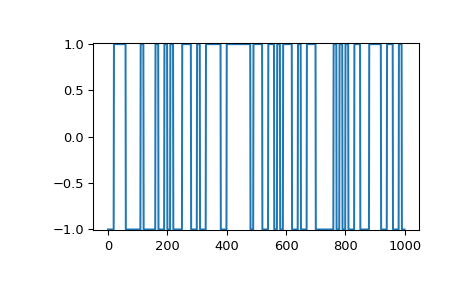
sk_dsp_comm.sigsys.NRZ_bits(N_bits, Ns, pulse='rect', alpha=0.25, M=6)[source]¶ Generate non-return-to-zero (NRZ) data bits with pulse shaping.
A baseband digital data signal using +/-1 amplitude signal values and including pulse shaping.
Parameters: - N_bits : number of NRZ +/-1 data bits to produce
- Ns : the number of samples per bit,
- pulse_type : ‘rect’ , ‘rc’, ‘src’ (default ‘rect’)
- alpha : excess bandwidth factor(default 0.25)
- M : single sided pulse duration (default = 6)
Returns: - x : ndarray of the NRZ signal values
- b : ndarray of the pulse shape
- data : ndarray of the underlying data bits
Notes
Pulse shapes include ‘rect’ (rectangular), ‘rc’ (raised cosine), ‘src’ (root raised cosine). The actual pulse length is 2*M+1 samples. This function is used by BPSK_tx in the Case Study article.
Examples
>>> import matplotlib.pyplot as plt
>>> from sk_dsp_comm.sigsys import NRZ_bits
>>> from numpy import arange
>>> x,b,data = NRZ_bits(100, 10)
>>> t = arange(len(x))
>>> plt.plot(t, x)
>>> plt.ylim([-1.01, 1.01])
>>> plt.show()
-
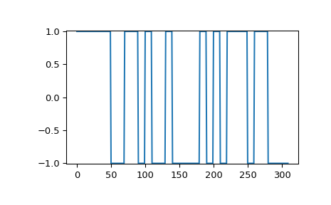
sk_dsp_comm.sigsys.NRZ_bits2(data, Ns, pulse='rect', alpha=0.25, M=6)[source]¶ Generate non-return-to-zero (NRZ) data bits with pulse shaping with user data
A baseband digital data signal using +/-1 amplitude signal values and including pulse shaping. The data sequence is user supplied.
Parameters: - data : ndarray of the data bits as 0/1 values
- Ns : the number of samples per bit,
- pulse_type : ‘rect’ , ‘rc’, ‘src’ (default ‘rect’)
- alpha : excess bandwidth factor(default 0.25)
- M : single sided pulse duration (default = 6)
Returns: - x : ndarray of the NRZ signal values
- b : ndarray of the pulse shape
Notes
Pulse shapes include ‘rect’ (rectangular), ‘rc’ (raised cosine), ‘src’ (root raised cosine). The actual pulse length is 2*M+1 samples.
Examples
>>> import matplotlib.pyplot as plt
>>> from sk_dsp_comm.sigsys import NRZ_bits2
>>> from sk_dsp_comm.sigsys import m_seq
>>> from numpy import arange
>>> x,b = NRZ_bits2(m_seq(5),10)
>>> t = arange(len(x))
>>> plt.ylim([-1.01, 1.01])
>>> plt.plot(t,x)
-
sk_dsp_comm.sigsys.OA_filter(x, h, N, mode=0)[source]¶ Overlap and add transform domain FIR filtering.
This function implements the classical overlap and add method of transform domain filtering using a length P FIR filter.
Parameters: - x : input signal to be filtered as an ndarray
- h : FIR filter coefficients as an ndarray of length P
- N : FFT size > P, typically a power of two
- mode : 0 or 1, when 1 returns a diagnostic matrix
Returns: - y : the filtered output as an ndarray
- y_mat : an ndarray whose rows are the individual overlap outputs.
Notes
y_mat is used for diagnostics and to gain understanding of the algorithm.
Examples
>>> import numpy as np
>>> from sk_dsp_comm.sigsys import OA_filter
>>> n = np.arange(0,100)
>>> x = np.cos(2*pi*0.05*n)
>>> b = np.ones(10)
>>> y = OA_filter(x,h,N)
>>> # set mode = 1
>>> y, y_mat = OA_filter(x,h,N,1)
-
sk_dsp_comm.sigsys.OS_filter(x, h, N, mode=0)[source]¶ Overlap and save transform domain FIR filtering.
This function implements the classical overlap and save method of transform domain filtering using a length P FIR filter.
Parameters: - x : input signal to be filtered as an ndarray
- h : FIR filter coefficients as an ndarray of length P
- N : FFT size > P, typically a power of two
- mode : 0 or 1, when 1 returns a diagnostic matrix
Returns: - y : the filtered output as an ndarray
- y_mat : an ndarray whose rows are the individual overlap outputs.
Notes
y_mat is used for diagnostics and to gain understanding of the algorithm.
Examples
>>> n = arange(0,100)
>>> x = cos(2*pi*0.05*n)
>>> b = ones(10)
>>> y = OS_filter(x,h,N)
>>> # set mode = 1
>>> y, y_mat = OS_filter(x,h,N,1)
-
sk_dsp_comm.sigsys.PN_gen(N_bits, m=5)[source]¶ Maximal length sequence signal generator.
Generates a sequence 0/1 bits of N_bit duration. The bits themselves are obtained from an m-sequence of length m. Available m-sequence (PN generators) include m = 2,3,…,12, & 16.
Parameters: - N_bits : the number of bits to generate
- m : the number of shift registers. 2,3, .., 12, & 16
Returns: - PN : ndarray of the generator output over N_bits
Notes
The sequence is periodic having period 2**m - 1 (2^m - 1).
Examples
>>> # A 15 bit period signal nover 50 bits
>>> PN = PN_gen(50,4)
-
sk_dsp_comm.sigsys.am_rx(x192)[source]¶ AM envelope detector receiver for the Chapter 17 Case Study
The receiver bandpass filter is not included in this function.
Parameters: - x192 : ndarray of the AM signal at sampling rate 192 ksps
Returns: - m_rx8 : ndarray of the demodulated message at 8 ksps
- t8 : ndarray of the time axis at 8 ksps
- m_rx192 : ndarray of the demodulated output at 192 ksps
- x_edet192 : ndarray of the envelope detector output at 192 ksps
Notes
The bandpass filter needed at the receiver front-end can be designed using b_bpf,a_bpf =
am_rx_BPF().Examples
>>> import numpy as np
>>> n = np.arange(0,1000)
>>> # 1 kHz message signal
>>> m = np.cos(2*np.pi*1000/8000.*n)
>>> m_rx8,t8,m_rx192,x_edet192 = am_rx(x192)
-
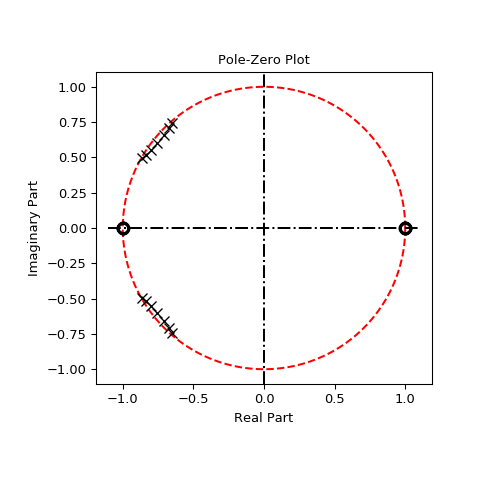
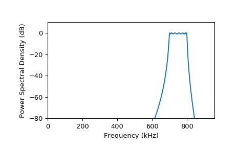
sk_dsp_comm.sigsys.am_rx_BPF(N_order=7, ripple_dB=1, B=10000.0, fs=192000.0)[source]¶ Bandpass filter design for the AM receiver Case Study of Chapter 17.
Design a 7th-order Chebyshev type 1 bandpass filter to remove/reduce adjacent channel intereference at the envelope detector input.
Parameters: - N_order : the filter order (default = 7)
- ripple_dB : the passband ripple in dB (default = 1)
- B : the RF bandwidth (default = 10e3)
- fs : the sampling frequency
Returns: - b_bpf : ndarray of the numerator filter coefficients
- a_bpf : ndarray of the denominator filter coefficients
Examples
>>> from scipy import signal
>>> import numpy as np
>>> import matplotlib.pyplot as plt
>>> import sk_dsp_comm.sigsys as ss
>>> # Use the default values
>>> b_bpf,a_bpf = ss.am_rx_BPF()
Pole-zero plot of the filter.
>>> ss.zplane(b_bpf,a_bpf)
>>> plt.show()
Plot of the frequency response.
>>> f = np.arange(0,192/2.,.1)
>>> w, Hbpf = signal.freqz(b_bpf,a_bpf,2*np.pi*f/192)
>>> plt.plot(f*10,20*np.log10(abs(Hbpf)))
>>> plt.axis([0,1920/2.,-80,10])
>>> plt.ylabel("Power Spectral Density (dB)")
>>> plt.xlabel("Frequency (kHz)")
>>> plt.show()
-
sk_dsp_comm.sigsys.am_tx(m, a_mod, fc=75000.0)[source]¶ AM transmitter for Case Study of Chapter 17.
Assume input is sampled at 8 Ksps and upsampling by 24 is performed to arrive at fs_out = 192 Ksps.
Parameters: - m : ndarray of the input message signal
- a_mod : AM modulation index, between 0 and 1
- fc : the carrier frequency in Hz
Returns: - x192 : ndarray of the upsampled by 24 and modulated carrier
- t192 : ndarray of the upsampled by 24 time axis
- m24 : ndarray of the upsampled by 24 message signal
Notes
The sampling rate of the input signal is assumed to be 8 kHz.
Examples
>>> n = arange(0,1000)
>>> # 1 kHz message signal
>>> m = cos(2*pi*1000/8000.*n)
>>> x192, t192 = am_tx(m,0.8,fc=75e3)
-
sk_dsp_comm.sigsys.biquad2(w_num, r_num, w_den, r_den)[source]¶ A biquadratic filter in terms of conjugate pole and zero pairs.
Parameters: - w_num : zero frequency (angle) in rad/sample
- r_num : conjugate zeros radius
- w_den : pole frequency (angle) in rad/sample
- r_den : conjugate poles radius; less than 1 for stability
Returns: - b : ndarray of numerator coefficients
- a : ndarray of denominator coefficients
Examples
>>> b,a = biquad2(pi/4., 1, pi/4., 0.95)
-
sk_dsp_comm.sigsys.bit_errors(z, data, start, Ns)[source]¶ A simple bit error counting function.
In its present form this function counts bit errors between hard decision BPSK bits in +/-1 form and compares them with 0/1 binary data that was transmitted. Timing between the Tx and Rx data is the responsibility of the user. An enhanced version of this function, which features automatic synching will be created in the future.
Parameters: - z : ndarray of hard decision BPSK data prior to symbol spaced sampling
- data : ndarray of reference bits in 1/0 format
- start : timing reference for the received
- Ns : the number of samples per symbol
Returns: - Pe_hat : the estimated probability of a bit error
Notes
The Tx and Rx data streams are exclusive-or’d and the then the bit errors are summed, and finally divided by the number of bits observed to form an estimate of the bit error probability. This function needs to be enhanced to be more useful.
Examples
>>> from scipy import signal
>>> x,b, data = NRZ_bits(1000,10)
>>> # set Eb/N0 to 8 dB
>>>  y = cpx_AWGN(x,8,10)
>>> # matched filter the signal
>>> z = signal.lfilter(b,1,y)
>>> # make bit decisions at 10 and Ns multiples thereafter
>>> Pe_hat = bit_errors(z,data,10,10)
-
sk_dsp_comm.sigsys.cascade_filters(b1, a1, b2, a2)[source]¶ Cascade two IIR digital filters into a single (b,a) coefficient set.
To cascade two digital filters (system functions) given their numerator and denominator coefficients you simply convolve the coefficient arrays.
Parameters: - b1 : ndarray of numerator coefficients for filter 1
- a1 : ndarray of denominator coefficients for filter 1
- b2 : ndarray of numerator coefficients for filter 2
- a2 : ndarray of denominator coefficients for filter 2
Returns: - b : ndarray of numerator coefficients for the cascade
- a : ndarray of denominator coefficients for the cascade
Examples
>>> from scipy import signal
>>> b1,a1 = signal.butter(3, 0.1)
>>> b2,a2 = signal.butter(3, 0.15)
>>> b,a = cascade_filters(b1,a1,b2,a2)
-
sk_dsp_comm.sigsys.conv_integral(x1, tx1, x2, tx2, extent=('f', 'f'))[source]¶ Continuous-time convolution of x1 and x2 with proper tracking of the output time axis.
Appromimate the convolution integral for the convolution of two continuous-time signals using the SciPy function signal. The time (sequence axis) are managed from input to output. y(t) = x1(t)*x2(t).
Parameters: - x1 : ndarray of signal x1 corresponding to tx1
- tx1 : ndarray time axis for x1
- x2 : ndarray of signal x2 corresponding to tx2
- tx2 : ndarray time axis for x2
- extent : (‘e1’,’e2’) where ‘e1’, ‘e2’ may be ‘f’ finite, ‘r’ right-sided, or ‘l’ left-sided
Returns: - y : ndarray of output values y
- ty : ndarray of the corresponding time axis for y
Notes
The output time axis starts at the sum of the starting values in x1 and x2 and ends at the sum of the two ending values in x1 and x2. The time steps used in x1(t) and x2(t) must match. The default extents of (‘f’,’f’) are used for signals that are active (have support) on or within t1 and t2 respectively. A right-sided signal such as exp(-a*t)*u(t) is semi-infinite, so it has extent ‘r’ and the convolution output will be truncated to display only the valid results.
Examples
>>> import matplotlib.pyplot as plt
>>> import numpy as np
>>> import sk_dsp_comm.sigsys as ss
>>> tx = np.arange(-5,10,.01)
>>> x = ss.rect(tx-2,4) # pulse starts at t = 0
>>> y,ty = ss.conv_integral(x,tx,x,tx)
>>> plt.plot(ty,y) # expect a triangle on [0,8]
>>> plt.show()
Now, consider a pulse convolved with an exponential.
>>> h = 4*np.exp(-4*tx)*ss.step(tx)
>>> y,ty = ss.conv_integral(x,tx,h,tx,extent=('f','r')) # note extents set
>>> plt.plot(ty,y) # expect a pulse charge and discharge waveform
-
sk_dsp_comm.sigsys.conv_sum(x1, nx1, x2, nx2, extent=('f', 'f'))[source]¶ Discrete convolution of x1 and x2 with proper tracking of the output time axis.
Convolve two discrete-time signals using the SciPy function
scipy.signal.convolution(). The time (sequence axis) are managed from input to output. y[n] = x1[n]*x2[n].Parameters: - x1 : ndarray of signal x1 corresponding to nx1
- nx1 : ndarray time axis for x1
- x2 : ndarray of signal x2 corresponding to nx2
- nx2 : ndarray time axis for x2
- extent : (‘e1’,’e2’) where ‘e1’, ‘e2’ may be ‘f’ finite, ‘r’ right-sided, or ‘l’ left-sided
Returns: - y : ndarray of output values y
- ny : ndarray of the corresponding sequence index n
Notes
The output time axis starts at the sum of the starting values in x1 and x2 and ends at the sum of the two ending values in x1 and x2. The default extents of (‘f’,’f’) are used for signals that are active (have support) on or within n1 and n2 respectively. A right-sided signal such as a^n*u[n] is semi-infinite, so it has extent ‘r’ and the convolution output will be truncated to display only the valid results.
Examples
>>> import matplotlib.pyplot as plt
>>> import numpy as np
>>> import sk_dsp_comm.sigsys as ss
>>> nx = np.arange(-5,10)
>>> x = ss.drect(nx,4)
>>> y,ny = ss.conv_sum(x,nx,x,nx)
>>> plt.stem(ny,y)
>>> plt.show()
Consider a pulse convolved with an exponential. (‘r’ type extent)
>>> h = 0.5**nx*ss.dstep(nx)
>>> y,ny = ss.conv_sum(x,nx,h,nx,('f','r')) # note extents set
>>> plt.stem(ny,y) # expect a pulse charge and discharge sequence
-
sk_dsp_comm.sigsys.cpx_AWGN(x, EsN0, Ns)[source]¶ Apply white Gaussian noise to a digital communications signal.
This function represents a complex baseband white Gaussian noise digital communications channel. The input signal array may be real or complex.
Parameters: - x : ndarray noise free complex baseband input signal.
- EsNO : set the channel Es/N0 (Eb/N0 for binary) level in dB
- Ns : number of samples per symbol (bit)
Returns: - y : ndarray x with additive noise added.
Notes
Set the channel energy per symbol-to-noise power spectral density ratio (Es/N0) in dB.
Examples
>>> x,b, data = NRZ_bits(1000,10)
>>> # set Eb/N0 = 10 dB
>>> y = cpx_AWGN(x,10,10)
-
sk_dsp_comm.sigsys.cruise_control(wn, zeta, T, vcruise, vmax, tf_mode='H')[source]¶ Cruise control with PI controller and hill disturbance.
This function returns various system function configurations for a the cruise control Case Study example found in the supplementary article. The plant model is obtained by the linearizing the equations of motion and the controller contains a proportional and integral gain term set via the closed-loop parameters natuarl frequency wn (rad/s) and damping zeta.
Parameters: - wn : closed-loop natural frequency in rad/s, nominally 0.1
- zeta : closed-loop damping factor, nominally 1.0
- T : vehicle time constant, nominally 10 s
- vcruise : cruise velocity set point, nominally 75 mph
- vmax : maximum vehicle velocity, nominally 120 mph
- tf_mode : ‘H’, ‘HE’, ‘HVW’, or ‘HED’ controls the system function returned by the function
- ‘H’ : closed-loop system function V(s)/R(s)
- ‘HE’ : closed-loop system function E(s)/R(s)
- ‘HVW’ : closed-loop system function V(s)/W(s)
- ‘HED’ : closed-loop system function E(s)/D(s), where D is the hill disturbance input
Returns: - b : numerator coefficient ndarray
- a : denominator coefficient ndarray
Examples
>>> # return the closed-loop system function output/input velocity
>>> b,a = cruise_control(wn,zeta,T,vcruise,vmax,tf_mode='H')
>>> # return the closed-loop system function loop error/hill disturbance
>>> b,a = cruise_control(wn,zeta,T,vcruise,vmax,tf_mode='HED')
-
sk_dsp_comm.sigsys.deci24(x)[source]¶ Decimate by L = 24 using Butterworth filters.
The decimation is done using two three stages. Downsample sample by L = 2 and lowpass filter, downsample by 3 and lowpass filter, then downsample by L = 4 and lowpass filter. In all cases the lowpass filter is a 10th-order Butterworth lowpass.
Parameters: - x : ndarray of the input signal
Returns: - y : ndarray of the output signal
Notes
The cutoff frequency of the lowpass filters is 1/2, 1/3, and 1/4 to track the upsampling by 2, 3, and 4 respectively.
Examples
>>> y = deci24(x)
-
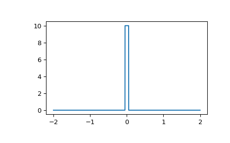
sk_dsp_comm.sigsys.delta_eps(t, eps)[source]¶ Rectangular pulse approximation to impulse function.
Parameters: - t : ndarray of time axis
- eps : pulse width
Returns: - d : ndarray containing the impulse approximation
Examples
>>> import matplotlib.pyplot as plt
>>> from numpy import arange
>>> from sk_dsp_comm.sigsys import delta_eps
>>> t = np.arange(-2,2,.001)
>>> d = delta_eps(t,.1)
>>> plt.plot(t,d)
>>> plt.show()
-
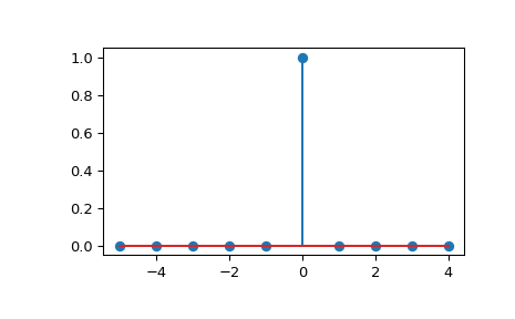
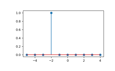
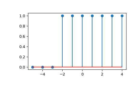
sk_dsp_comm.sigsys.dimpulse(n)[source]¶ Discrete impulse function delta[n].
Parameters: - n : ndarray of the time axis
Returns: - x : ndarray of the signal delta[n]
Examples
>>> import matplotlib.pyplot as plt
>>> from numpy import arange
>>> from sk_dsp_comm.sigsys import dimpulse
>>> n = arange(-5,5)
>>> x = dimpulse(n)
>>> plt.stem(n,x)
>>> plt.show()
Shift the delta left by 2.
>>> x = dimpulse(n+2)
>>> plt.stem(n,x)
-
sk_dsp_comm.sigsys.downsample(x, M, p=0)[source]¶ Downsample by factor M
Keep every Mth sample of the input. The phase of the input samples kept can be selected.
Parameters: - x : ndarray of input signal values
- M : downsample factor
- p : phase of decimated value, 0 (default), 1, …, M-1
Returns: - y : ndarray of the output signal values
Examples
>>> y = downsample(x,3)
>>> y = downsample(x,3,1)
-
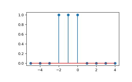
sk_dsp_comm.sigsys.drect(n, N)[source]¶ Discrete rectangle function of duration N samples.
The signal is active on the interval 0 <= n <= N-1. Also known as the rectangular window function, which is available in scipy.signal.
Parameters: - n : ndarray of the time axis
- N : the pulse duration
Returns: - x : ndarray of the signal
Notes
The discrete rectangle turns on at n = 0, off at n = N-1 and has duration of exactly N samples.
Examples
>>> import matplotlib.pyplot as plt
>>> from numpy import arange
>>> from sk_dsp_comm.sigsys import drect
>>> n = arange(-5,5)
>>> x = drect(n, N=3)
>>> plt.stem(n,x)
>>> plt.show()
Shift the delta left by 2.
>>> x = drect(n+2, N=3)
>>> plt.stem(n,x)
-
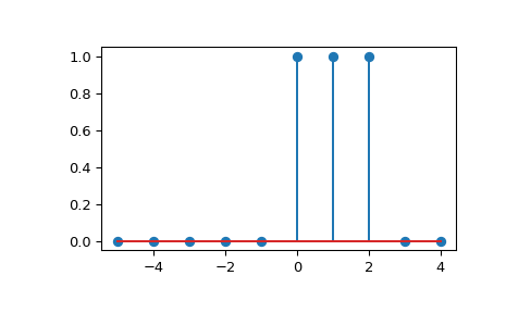
sk_dsp_comm.sigsys.dstep(n)[source]¶ Discrete step function u[n].
Parameters: - n : ndarray of the time axis
Returns: - x : ndarray of the signal u[n]
Examples
>>> import matplotlib.pyplot as plt
>>> from numpy import arange
>>> from sk_dsp_comm.sigsys import dstep
>>> n = arange(-5,5)
>>> x = dstep(n)
>>> plt.stem(n,x)
>>> plt.show()
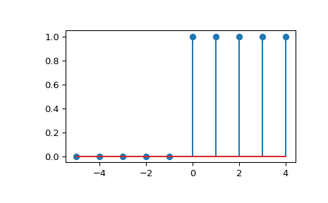
Shift the delta left by 2.
>>> x = dstep(n+2)
>>> plt.stem(n,x)
-
sk_dsp_comm.sigsys.env_det(x)[source]¶ Ideal envelope detector.
This function retains the positive half cycles of the input signal.
Parameters: - x : ndarray of the input sugnal
Returns: - y : ndarray of the output signal
Examples
>>> n = arange(0,100)
>>> # 1 kHz message signal
>>> m = cos(2*pi*1000/8000.*n)
>>> x192, t192, m24 = am_tx(m,0.8,fc=75e3)
>>> y = env_det(x192)
-
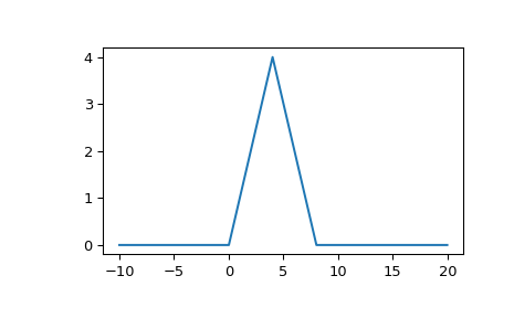
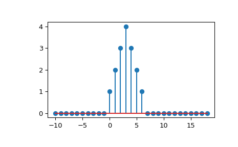
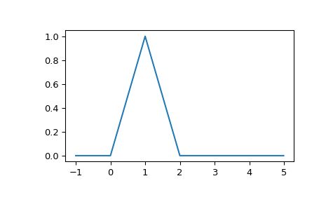
sk_dsp_comm.sigsys.ex6_2(n)[source]¶ Generate a triangle pulse as described in Example 6-2 of Chapter 6.
You need to supply an index array n that covers at least [-2, 5]. The function returns the hard-coded signal of the example.
Parameters: - n : time index ndarray covering at least -2 to +5.
Returns: - x : ndarray of signal samples in x
Examples
>>> import numpy as np
>>> import matplotlib.pyplot as plt
>>> from sk_dsp_comm import sigsys as ss
>>> n = np.arange(-5,8)
>>> x = ss.ex6_2(n)
>>> plt.stem(n,x) # creates a stem plot of x vs n
-
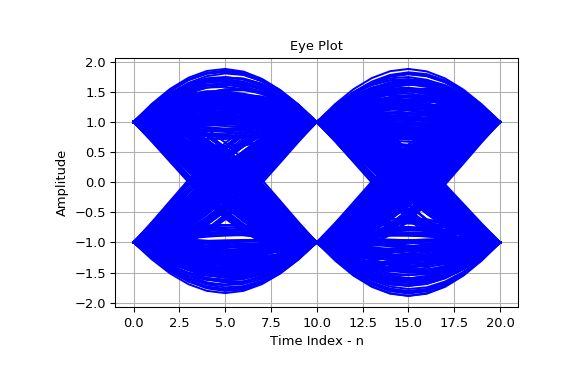
sk_dsp_comm.sigsys.eye_plot(x, L, S=0)[source]¶ Eye pattern plot of a baseband digital communications waveform.
The signal must be real, but can be multivalued in terms of the underlying modulation scheme. Used for BPSK eye plots in the Case Study article.
Parameters: - x : ndarray of the real input data vector/array
- L : display length in samples (usually two symbols)
- S : start index
Returns: - Nothing : A plot window opens containing the eye plot
Notes
Increase S to eliminate filter transients.
Examples
1000 bits at 10 samples per bit with ‘rc’ shaping.
>>> import matplotlib.pyplot as plt
>>> from sk_dsp_comm import sigsys as ss
>>> x,b, data = ss.NRZ_bits(1000,10,'rc')
>>> ss.eye_plot(x,20,60)
-
sk_dsp_comm.sigsys.fir_iir_notch(fi, fs, r=0.95)[source]¶ Design a second-order FIR or IIR notch filter.
A second-order FIR notch filter is created by placing conjugate zeros on the unit circle at angle corresponidng to the notch center frequency. The IIR notch variation places a pair of conjugate poles at the same angle, but with radius r < 1 (typically 0.9 to 0.95).
Parameters: - fi : notch frequency is Hz relative to fs
- fs : the sampling frequency in Hz, e.g. 8000
- r : pole radius for IIR version, default = 0.95
Returns: - b : numerator coefficient ndarray
- a : denominator coefficient ndarray
Notes
If the pole radius is 0 then an FIR version is created, that is there are no poles except at z = 0.
Examples
>>> import matplotlib.pyplot as plt
>>> from sk_dsp_comm import sigsys as ss
>>> b_FIR, a_FIR = ss.fir_iir_notch(1000,8000,0)
>>> ss.zplane(b_FIR, a_FIR)
>>> plt.show()
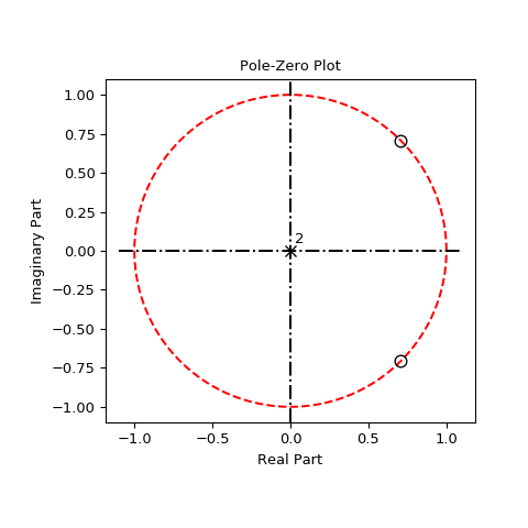
>>> b_IIR, a_IIR = ss.fir_iir_notch(1000,8000)
>>> ss.zplane(b_IIR, a_IIR)
-
sk_dsp_comm.sigsys.from_wav(filename)[source]¶ Read a wave file.
A wrapper function for scipy.io.wavfile.read that also includes int16 to float [-1,1] scaling.
Parameters: - filename : file name string
Returns: - fs : sampling frequency in Hz
- x : ndarray of normalized to 1 signal samples
Examples
>>> fs,x = from_wav('test_file.wav')
-
sk_dsp_comm.sigsys.fs_approx(Xk, fk, t)[source]¶ Synthesize periodic signal x(t) using Fourier series coefficients at harmonic frequencies
Assume the signal is real so coefficients Xk are supplied for nonnegative indicies. The negative index coefficients are assumed to be complex conjugates.
Parameters: - Xk : ndarray of complex Fourier series coefficients
- fk : ndarray of harmonic frequencies in Hz
- t : ndarray time axis corresponding to output signal array x_approx
Returns: - x_approx : ndarray of periodic waveform approximation over time span t
Examples
>>> t = arange(0,2,.002)
>>> # a 20% duty cycle pulse train
>>> n = arange(0,20,1) # 0 to 19th harmonic
>>> fk = 1*n % period = 1s
>>> t, x_approx = fs_approx(Xk,fk,t)
>>> plot(t,x_approx)
-
sk_dsp_comm.sigsys.fs_coeff(xp, N, f0, one_side=True)[source]¶ Numerically approximate the Fourier series coefficients given periodic x(t).
The input is assummed to represent one period of the waveform x(t) that has been uniformly sampled. The number of samples supplied to represent one period of the waveform sets the sampling rate.
Parameters: - xp : ndarray of one period of the waveform x(t)
- N : maximum Fourier series coefficient, [0,…,N]
- f0 : fundamental frequency used to form fk.
Returns: - Xk : ndarray of the coefficients over indices [0,1,…,N]
- fk : ndarray of the harmonic frequencies [0, f0,2f0,…,Nf0]
Notes
len(xp) >= 2*N+1 as len(xp) is the fft length.
Examples
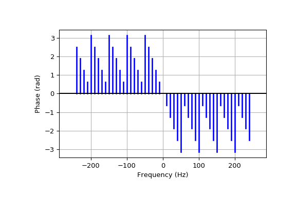
>>> import matplotlib.pyplot as plt
>>> from numpy import arange
>>> import sk_dsp_comm.sigsys as ss
>>> t = arange(0,1,1/1024.)
>>> # a 20% duty cycle pulse starting at t = 0
>>> x_rect = ss.rect(t-.1,0.2)
>>> Xk, fk = ss.fs_coeff(x_rect,25,10)
>>> # plot the spectral lines
>>> ss.line_spectra(fk,Xk,'mag')
>>> plt.show()
-
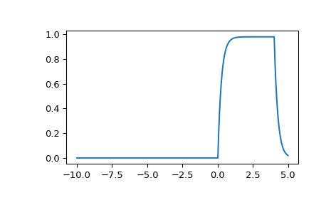
sk_dsp_comm.sigsys.ft_approx(x, t, Nfft)[source]¶ Approximate the Fourier transform of a finite duration signal using scipy.signal.freqz()
Parameters: - x : input signal array
- t : time array used to create x(t)
- Nfft : the number of frdquency domain points used to
approximate X(f) on the interval [fs/2,fs/2], where fs = 1/Dt. Dt being the time spacing in array t
Returns: - f : frequency axis array in Hz
- X : the Fourier transform approximation (complex)
Notes
The output time axis starts at the sum of the starting values in x1 and x2 and ends at the sum of the two ending values in x1 and x2. The default extents of (‘f’,’f’) are used for signals that are active (have support) on or within n1 and n2 respectively. A right-sided signal such as \(a^n*u[n]\) is semi-infinite, so it has extent ‘r’ and the convolution output will be truncated to display only the valid results.
Examples
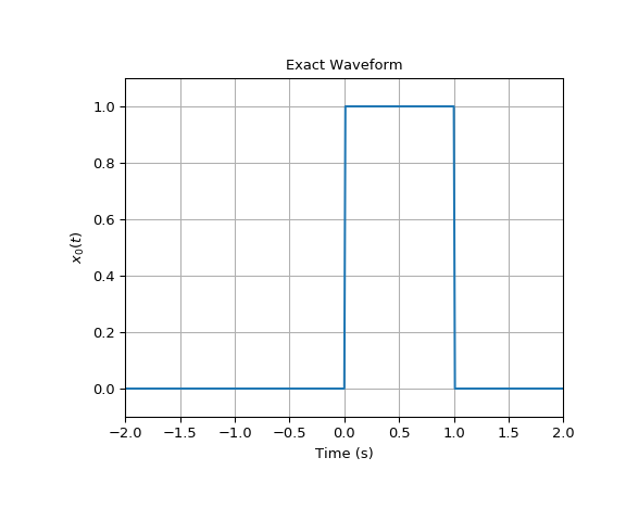
>>> import matplotlib.pyplot as plt
>>> import numpy as np
>>> import sk_dsp_comm.sigsys as ss
>>> fs = 100 # sampling rate in Hz
>>> tau = 1
>>> t = np.arange(-5,5,1/fs)
>>> x0 = ss.rect(t-.5,tau)
>>> plt.figure(figsize=(6,5))
>>> plt.plot(t,x0)
>>> plt.grid()
>>> plt.ylim([-0.1,1.1])
>>> plt.xlim([-2,2])
>>> plt.title(r'Exact Waveform')
>>> plt.xlabel(r'Time (s)')
>>> plt.ylabel(r'$x_0(t)$')
>>> plt.show()
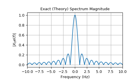
>>> # FT Exact Plot
>>> import matplotlib.pyplot as plt
>>> import numpy as np
>>> import sk_dsp_comm.sigsys as ss
>>> fs = 100 # sampling rate in Hz
>>> tau = 1
>>> t = np.arange(-5,5,1/fs)
>>> x0 = ss.rect(t-.5,tau)
>>> fe = np.arange(-10,10,.01)
>>> X0e = tau*np.sinc(fe*tau)
>>> plt.plot(fe,abs(X0e))
>>> #plot(f,angle(X0))
>>> plt.grid()
>>> plt.xlim([-10,10])
>>> plt.title(r'Exact (Theory) Spectrum Magnitude')
>>> plt.xlabel(r'Frequency (Hz)')
>>> plt.ylabel(r'$|X_0e(f)|$')
>>> plt.show()
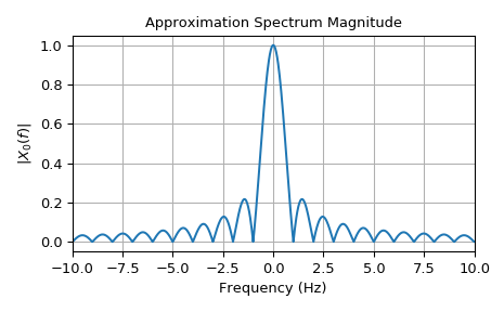
>>> # FT Approximation Plot
>>> import matplotlib.pyplot as plt
>>> import numpy as np
>>> import sk_dsp_comm.sigsys as ss
>>> fs = 100 # sampling rate in Hz
>>> tau = 1
>>> t = np.arange(-5,5,1/fs)
>>> x0 = ss.rect(t-.5,tau)
>>> f,X0 = ss.ft_approx(x0,t,4096)
>>> plt.plot(f,abs(X0))
>>> #plt.plot(f,angle(X0))
>>> plt.grid()
>>> plt.xlim([-10,10])
>>> plt.title(r'Approximation Spectrum Magnitude')
>>> plt.xlabel(r'Frequency (Hz)')
>>> plt.ylabel(r'$|X_0(f)|$');
>>> plt.tight_layout()
>>> plt.show()
-
sk_dsp_comm.sigsys.interp24(x)[source]¶ Interpolate by L = 24 using Butterworth filters.
The interpolation is done using three stages. Upsample by L = 2 and lowpass filter, upsample by 3 and lowpass filter, then upsample by L = 4 and lowpass filter. In all cases the lowpass filter is a 10th-order Butterworth lowpass.
Parameters: - x : ndarray of the input signal
Returns: - y : ndarray of the output signal
Notes
The cutoff frequency of the lowpass filters is 1/2, 1/3, and 1/4 to track the upsampling by 2, 3, and 4 respectively.
Examples
>>> y = interp24(x)
-
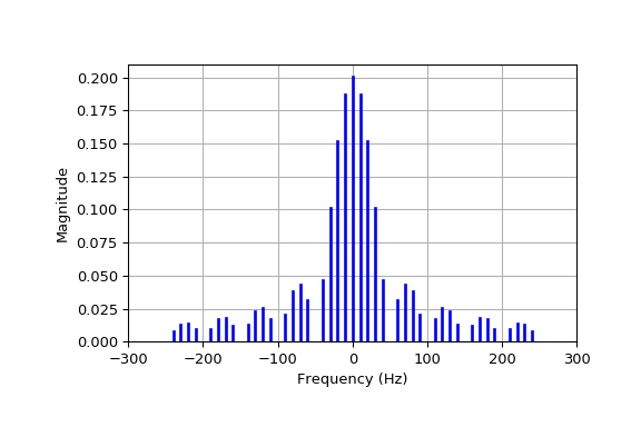
sk_dsp_comm.sigsys.line_spectra(fk, Xk, mode, sides=2, linetype='b', lwidth=2, floor_dB=-100, fsize=(6, 4))[source]¶ Plot the Fouier series line spectral given the coefficients.
This function plots two-sided and one-sided line spectra of a periodic signal given the complex exponential Fourier series coefficients and the corresponding harmonic frequencies.
Parameters: - fk : vector of real sinusoid frequencies
- Xk : magnitude and phase at each positive frequency in fk
- mode : ‘mag’ => magnitude plot, ‘magdB’ => magnitude in dB plot,
- mode cont : ‘magdBn’ => magnitude in dB normalized, ‘phase’ => a phase plot in radians
- sides : 2; 2-sided or 1-sided
- linetype : line type per Matplotlib definitions, e.g., ‘b’;
- lwidth : 2; linewidth in points
- fsize : optional figure size in inches, default = (6,4) inches
Returns: - Nothing : A plot window opens containing the line spectrum plot
Notes
Since real signals are assumed the frequencies of fk are 0 and/or positive numbers. The supplied Fourier coefficients correspond.
Examples
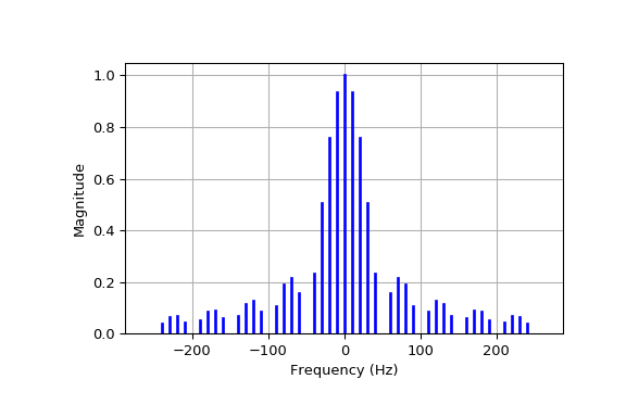
>>> import matplotlib.pyplot as plt
>>> import numpy as np
>>> from sk_dsp_comm.sigsys import line_spectra
>>> n = np.arange(0,25)
>>> # a pulse train with 10 Hz fundamental and 20% duty cycle
>>> fk = n*10
>>> Xk = np.sinc(n*10*.02)*np.exp(-1j*2*np.pi*n*10*.01) # 1j = sqrt(-1)
>>> line_spectra(fk,Xk,'mag')
>>> plt.show()
>>> line_spectra(fk,Xk,'phase')
-
sk_dsp_comm.sigsys.lms_ic(r, M, mu, delta=1)[source]¶ Least mean square (LMS) interference canceller adaptive filter.
A complete LMS adaptive filter simulation function for the case of interference cancellation. Used in the digital filtering case study.
Parameters: - M : FIR Filter length (order M-1)
- delta : Delay used to generate the reference signal
- mu : LMS step-size
- delta : decorrelation delay between input and FIR filter input
Returns: - n : ndarray Index vector
- r : ndarray noisy (with interference) input signal
- r_hat : ndarray filtered output (NB_hat[n])
- e : ndarray error sequence (WB_hat[n])
- ao : ndarray final value of weight vector
- F : ndarray frequency response axis vector
- Ao : ndarray frequency response of filter
Examples
>>> # import a speech signal
>>> fs,s = from_wav('OSR_us_000_0030_8k.wav')
>>> # add interference at 1kHz and 1.5 kHz and
>>> # truncate to 5 seconds
>>> r = soi_snoi_gen(s,10,5*8000,[1000, 1500])
>>> # simulate with a 64 tap FIR and mu = 0.005
>>> n,r,r_hat,e,ao,F,Ao = lms_ic(r,64,0.005)
-
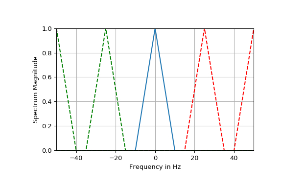
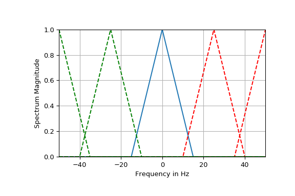
sk_dsp_comm.sigsys.lp_samp(fb, fs, fmax, N, shape='tri', fsize=(6, 4))[source]¶ Lowpass sampling theorem plotting function.
Display the spectrum of a sampled signal after setting the bandwidth, sampling frequency, maximum display frequency, and spectral shape.
Parameters: - fb : spectrum lowpass bandwidth in Hz
- fs : sampling frequency in Hz
- fmax : plot over [-fmax,fmax]
- shape : ‘tri’ or ‘line’
- N : number of translates, N positive and N negative
- fsize : the size of the figure window, default (6,4)
Returns: - Nothing : A plot window opens containing the spectrum plot
Examples
>>> import matplotlib.pyplot as plt
>>> from sk_dsp_comm.sigsys import lp_samp
No aliasing as bandwidth 10 Hz < 25/2; fs > fb.
>>> lp_samp(10,25,50,10)
>>> plt.show()
Now aliasing as bandwidth 15 Hz > 25/2; fs < fb.
>>> lp_samp(15,25,50,10)
-
sk_dsp_comm.sigsys.lp_tri(f, fb)[source]¶ Triangle spectral shape function used by
lp_samp().Parameters: - f : ndarray containing frequency samples
- fb : the bandwidth as a float constant
Returns: - x : ndarray of spectrum samples for a single triangle shape
Notes
This is a support function for the lowpass spectrum plotting function
lp_samp().Examples
>>> x = lp_tri(f, fb)
-
sk_dsp_comm.sigsys.m_seq(m)[source]¶ Generate an m-sequence ndarray using an all-ones initialization.
Available m-sequence (PN generators) include m = 2,3,…,12, & 16.
Parameters: - m : the number of shift registers. 2,3, .., 12, & 16
Returns: - c : ndarray of one period of the m-sequence
Notes
The sequence period is 2**m - 1 (2^m - 1).
Examples
>>> c = m_seq(5)
-
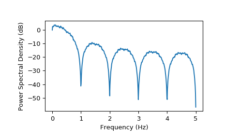
sk_dsp_comm.sigsys.my_psd(x, NFFT=1024, Fs=1)[source]¶ A local version of NumPy’s PSD function that returns the plot arrays.
A mlab.psd wrapper function that returns two ndarrays; makes no attempt to auto plot anything.
Parameters: - x : ndarray input signal
- NFFT : a power of two, e.g., 2**10 = 1024
- Fs : the sampling rate in Hz
Returns: - Px : ndarray of the power spectrum estimate
- f : ndarray of frequency values
Notes
This function makes it easier to overlay spectrum plots because you have better control over the axis scaling than when using psd() in the autoscale mode.
Examples
>>> import matplotlib.pyplot as plt
>>> from numpy import log10
>>> from sk_dsp_comm import sigsys as ss
>>> x,b, data = ss.NRZ_bits(10000,10)
>>> Px,f = ss.my_psd(x,2**10,10)
>>> plt.plot(f, 10*log10(Px))
>>> plt.ylabel("Power Spectral Density (dB)")
>>> plt.xlabel("Frequency (Hz)")
>>> plt.show()
-
sk_dsp_comm.sigsys.peaking(GdB, fc, Q=3.5, fs=44100.0)[source]¶ A second-order peaking filter having GdB gain at fc and approximately and 0 dB otherwise.
The filter coefficients returns correspond to a biquadratic system function containing five parameters.
Parameters: - GdB : Lowpass gain in dB
- fc : Center frequency in Hz
- Q : Filter Q which is inversely proportional to bandwidth
- fs : Sampling frquency in Hz
Returns: - b : ndarray containing the numerator filter coefficients
- a : ndarray containing the denominator filter coefficients
Examples
>>> import matplotlib.pyplot as plt
>>> import numpy as np
>>> from sk_dsp_comm.sigsys import peaking
>>> from scipy import signal
>>> b,a = peaking(2.0,500)
>>> f = np.logspace(1,5,400)
>>> w,H = signal.freqz(b,a,2*np.pi*f/44100)
>>> plt.semilogx(f,20*np.log10(abs(H)))
>>> plt.ylabel("Power Spectral Density (dB)")
>>> plt.xlabel("Frequency (Hz)")
>>> plt.show()
>>> b,a = peaking(-5.0,500,4)
>>> w,H = signal.freqz(b,a,2*np.pi*f/44100)
>>> plt.semilogx(f,20*np.log10(abs(H)))
>>> plt.ylabel("Power Spectral Density (dB)")
>>> plt.xlabel("Frequency (Hz)")
-
sk_dsp_comm.sigsys.position_CD(Ka, out_type='fb_exact')[source]¶ CD sled position control case study of Chapter 18.
The function returns the closed-loop and open-loop system function for a CD/DVD sled position control system. The loop amplifier gain is the only variable that may be changed. The returned system function can however be changed.
Parameters: - Ka : loop amplifier gain, start with 50.
- out_type : ‘open_loop’ for open loop system function
- out_type : ‘fb_approx’ for closed-loop approximation
- out_type : ‘fb_exact’ for closed-loop exact
Returns: - b : numerator coefficient ndarray
- a : denominator coefficient ndarray
Notes
With the exception of the loop amplifier gain, all other parameters are hard-coded from Case Study example.
Examples
>>> b,a = position_CD(Ka,'fb_approx')
>>> b,a = position_CD(Ka,'fb_exact')
-
sk_dsp_comm.sigsys.prin_alias(f_in, fs)[source]¶ Calculate the principle alias frequencies.
Given an array of input frequencies the function returns an array of principle alias frequencies.
Parameters: - f_in : ndarray of input frequencies
- fs : sampling frequency
Returns: - f_out : ndarray of principle alias frequencies
Examples
>>> # Linear frequency sweep from 0 to 50 Hz
>>> f_in = arange(0,50,0.1)
>>> # Calculate principle alias with fs = 10 Hz
>>> f_out = prin_alias(f_in,10)
-
sk_dsp_comm.sigsys.rc_imp(Ns, alpha, M=6)[source]¶ A truncated raised cosine pulse used in digital communications.
The pulse shaping factor \(0< \alpha < 1\) is required as well as the truncation factor M which sets the pulse duration to be 2*M*Tsymbol.
Parameters: - Ns : number of samples per symbol
- alpha : excess bandwidth factor on (0, 1), e.g., 0.35
- M : equals RC one-sided symbol truncation factor
Returns: - b : ndarray containing the pulse shape
Notes
The pulse shape b is typically used as the FIR filter coefficients when forming a pulse shaped digital communications waveform.
Examples
Ten samples per symbol and alpha = 0.35.
>>> import matplotlib.pyplot as plt
>>> from numpy import arange
>>> from sk_dsp_comm.sigsys import rc_imp
>>> b = rc_imp(10,0.35)
>>> n = arange(-10*6,10*6+1)
>>> plt.stem(n,b)
>>> plt.show()
-
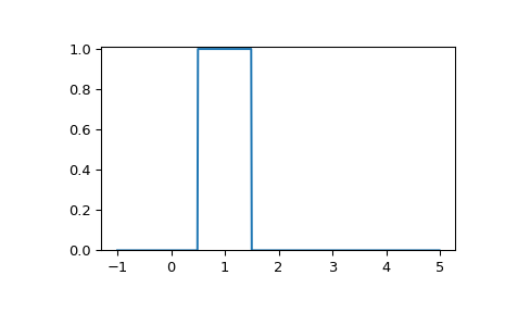
sk_dsp_comm.sigsys.rect(t, tau)[source]¶ Approximation to the rectangle pulse Pi(t/tau).
In this numerical version of Pi(t/tau) the pulse is active over -tau/2 <= t <= tau/2.
Parameters: - t : ndarray of the time axis
- tau : the pulse width
Returns: - x : ndarray of the signal Pi(t/tau)
Examples
>>> import matplotlib.pyplot as plt
>>> from numpy import arange
>>> from sk_dsp_comm.sigsys import rect
>>> t = arange(-1,5,.01)
>>> x = rect(t,1.0)
>>> plt.plot(t,x)
>>> plt.ylim([0, 1.01])
>>> plt.show()
To turn on the pulse at t = 1 shift t.
>>> x = rect(t - 1.0,1.0)
>>> plt.plot(t,x)
>>> plt.ylim([0, 1.01])
-
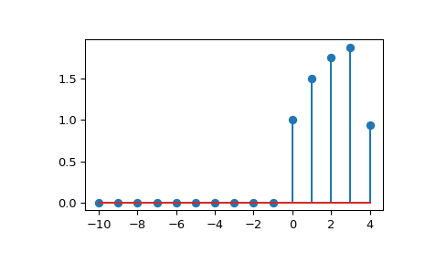
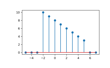
sk_dsp_comm.sigsys.rect_conv(n, N_len)[source]¶ The theoretical result of convolving two rectangle sequences.
The result is a triangle. The solution is based on pure analysis. Simply coded as opposed to efficiently coded.
Parameters: - n : ndarray of time axis
- N_len : rectangle pulse duration
Returns: - y : ndarray of of output signal
Examples
>>> import matplotlib.pyplot as plt
>>> from numpy import arange
>>> from sk_dsp_comm.sigsys import rect_conv
>>> n = arange(-5,20)
>>> y = rect_conv(n,6)
>>> plt.plot(n, y)
>>> plt.show()
-
sk_dsp_comm.sigsys.scatter(x, Ns, start)[source]¶ Sample a baseband digital communications waveform at the symbol spacing.
Parameters: - x : ndarray of the input digital comm signal
- Ns : number of samples per symbol (bit)
- start : the array index to start the sampling
Returns: - xI : ndarray of the real part of x following sampling
- xQ : ndarray of the imaginary part of x following sampling
Notes
Normally the signal is complex, so the scatter plot contains clusters at points in the complex plane. For a binary signal such as BPSK, the point centers are nominally +/-1 on the real axis. Start is used to eliminate transients from the FIR pulse shaping filters from appearing in the scatter plot.
Examples
>>> import matplotlib.pyplot as plt
>>> from sk_dsp_comm import sigsys as ss
>>> x,b, data = ss.NRZ_bits(1000,10,'rc')
>>> # Add some noise so points are now scattered about +/-1
>>> y = ss.cpx_AWGN(x,20,10)
>>> yI,yQ = ss.scatter(y,10,60)
>>> plt.plot(yI,yQ,'.')
>>> plt.axis('equal')
>>> plt.ylabel("Quadrature")
>>> plt.xlabel("In-Phase")
>>> plt.grid()
>>> plt.show()
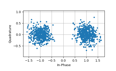
-
sk_dsp_comm.sigsys.simpleQuant(x, Btot, Xmax, Limit)[source]¶ A simple rounding quantizer for bipolar signals having Btot = B + 1 bits.
This function models a quantizer that employs Btot bits that has one of three selectable limiting types: saturation, overflow, and none. The quantizer is bipolar and implements rounding.
Parameters: - x : input signal ndarray to be quantized
- Btot : total number of bits in the quantizer, e.g. 16
- Xmax : quantizer full-scale dynamic range is [-Xmax, Xmax]
- Limit = Limiting of the form ‘sat’, ‘over’, ‘none’
Returns: - xq : quantized output ndarray
Notes
The quantization can be formed as e = xq - x
Examples
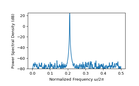
>>> import matplotlib.pyplot as plt
>>> from matplotlib.mlab import psd
>>> import numpy as np
>>> from sk_dsp_comm import sigsys as ss
>>> n = np.arange(0,10000)
>>> x = np.cos(2*np.pi*0.211*n)
>>> y = ss.sinusoidAWGN(x,90)
>>> Px, f = psd(y,2**10,Fs=1)
>>> plt.plot(f, 10*np.log10(Px))
>>> plt.ylim([-80, 25])
>>> plt.ylabel("Power Spectral Density (dB)")
>>> plt.xlabel(r'Normalized Frequency $\omega/2\pi$')
>>> plt.show()
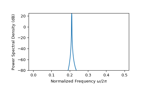
>>> yq = ss.simpleQuant(y,12,1,'sat')
>>> Px, f = psd(yq,2**10,Fs=1)
>>> plt.plot(f, 10*np.log10(Px))
>>> plt.ylim([-80, 25])
>>> plt.ylabel("Power Spectral Density (dB)")
>>> plt.xlabel(r'Normalized Frequency $\omega/2\pi$')
>>> plt.show()
-
sk_dsp_comm.sigsys.simple_SA(x, NS, NFFT, fs, NAVG=1, window='boxcar')[source]¶ Spectral estimation using windowing and averaging.
This function implements averaged periodogram spectral estimation estimation similar to the NumPy’s psd() function, but more specialized for the the windowing case study of Chapter 16.
Parameters: - x : ndarray containing the input signal
- NS : The subrecord length less zero padding, e.g. NS < NFFT
- NFFT : FFT length, e.g., 1024 = 2**10
- fs : sampling rate in Hz
- NAVG : the number of averages, e.g., 1 for deterministic signals
- window : hardcoded window ‘boxcar’ (default) or ‘hanning’
Returns: - f : ndarray frequency axis in Hz on [0, fs/2]
- Sx : ndarray the power spectrum estimate
Notes
The function also prints the maximum number of averages K possible for the input data record.
Examples
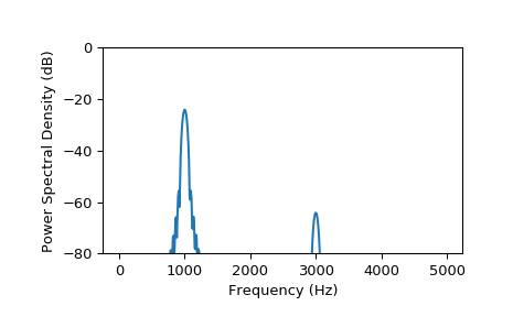
>>> import matplotlib.pyplot as plt
>>> import numpy as np
>>> from sk_dsp_comm import sigsys as ss
>>> n = np.arange(0,2048)
>>> x = np.cos(2*np.pi*1000/10000*n) + 0.01*np.cos(2*np.pi*3000/10000*n)
>>> f, Sx = ss.simple_SA(x,128,512,10000)
>>> plt.plot(f, 10*np.log10(Sx))
>>> plt.ylim([-80, 0])
>>> plt.xlabel("Frequency (Hz)")
>>> plt.ylabel("Power Spectral Density (dB)")
>>> plt.show()
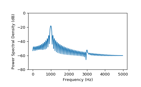
With a hanning window.
>>> f, Sx = ss.simple_SA(x,256,1024,10000,window='hanning')
>>> plt.plot(f, 10*np.log10(Sx))
>>> plt.xlabel("Frequency (Hz)")
>>> plt.ylabel("Power Spectral Density (dB)")
>>> plt.ylim([-80, 0])
-
sk_dsp_comm.sigsys.sinusoidAWGN(x, SNRdB)[source]¶ Add white Gaussian noise to a single real sinusoid.
Input a single sinusoid to this function and it returns a noisy sinusoid at a specific SNR value in dB. Sinusoid power is calculated using np.var.
Parameters: - x : Input signal as ndarray consisting of a single sinusoid
- SNRdB : SNR in dB for output sinusoid
Returns: - y : Noisy sinusoid return vector
Examples
>>> # set the SNR to 10 dB
>>> n = arange(0,10000)
>>> x = cos(2*pi*0.04*n)
>>> y = sinusoidAWGN(x,10.0)
-
sk_dsp_comm.sigsys.soi_snoi_gen(s, SIR_dB, N, fi, fs=8000)[source]¶ Add an interfering sinusoidal tone to the input signal at a given SIR_dB.
The input is the signal of interest (SOI) and number of sinsuoid signals not of interest (SNOI) are addedto the SOI at a prescribed signal-to- intereference SIR level in dB.
Parameters: - s : ndarray of signal of SOI
- SIR_dB : interference level in dB
- N : Trim input signal s to length N + 1 samples
- fi : ndarray of intereference frequencies in Hz
- fs : sampling rate in Hz, default is 8000 Hz
Returns: - r : ndarray of combined signal plus intereference of length N+1 samples
Examples
>>> # load a speech ndarray and trim to 5*8000 + 1 samples
>>> fs,s = from_wav('OSR_us_000_0030_8k.wav')
>>> r = soi_snoi_gen(s,10,5*8000,[1000, 1500])
-
sk_dsp_comm.sigsys.splane(b, a, auto_scale=True, size=[-1, 1, -1, 1])[source]¶ Create an s-plane pole-zero plot.
As input the function uses the numerator and denominator s-domain system function coefficient ndarrays b and a respectively. Assumed to be stored in descending powers of s.
Parameters: - b : numerator coefficient ndarray.
- a : denominator coefficient ndarray.
- auto_scale : True
- size : [xmin,xmax,ymin,ymax] plot scaling when scale = False
Returns: - (M,N) : tuple of zero and pole counts + plot window
Notes
This function tries to identify repeated poles and zeros and will place the multiplicity number above and to the right of the pole or zero. The difficulty is setting the tolerance for this detection. Currently it is set at 1e-3 via the function signal.unique_roots.
Examples
>>> # Here the plot is generated using auto_scale
>>> splane(b,a)
>>> # Here the plot is generated using manual scaling
>>> splane(b,a,False,[-10,1,-10,10])
-
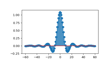
sk_dsp_comm.sigsys.sqrt_rc_imp(Ns, alpha, M=6)[source]¶ A truncated square root raised cosine pulse used in digital communications.
The pulse shaping factor 0< alpha < 1 is required as well as the truncation factor M which sets the pulse duration to be 2*M*Tsymbol.
Parameters: - Ns : number of samples per symbol
- alpha : excess bandwidth factor on (0, 1), e.g., 0.35
- M : equals RC one-sided symbol truncation factor
Returns: - b : ndarray containing the pulse shape
Notes
The pulse shape b is typically used as the FIR filter coefficients when forming a pulse shaped digital communications waveform. When square root raised cosine (SRC) pulse is used generate Tx signals and at the receiver used as a matched filter (receiver FIR filter), the received signal is now raised cosine shaped, this having zero intersymbol interference and the optimum removal of additive white noise if present at the receiver input.
Examples
>>> # ten samples per symbol and alpha = 0.35
>>> import matplotlib.pyplot as plt
>>> from numpy import arange
>>> from sk_dsp_comm.sigsys import sqrt_rc_imp
>>> b = sqrt_rc_imp(10,0.35)
>>> n = arange(-10*6,10*6+1)
>>> plt.stem(n,b)
>>> plt.show()
-
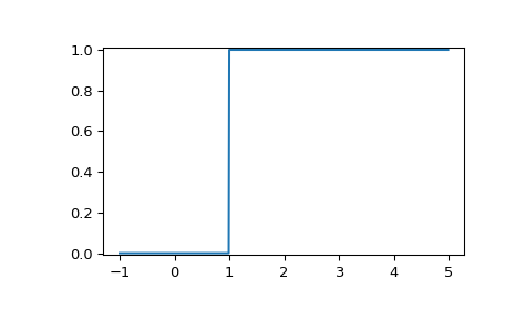
sk_dsp_comm.sigsys.step(t)[source]¶ Approximation to step function signal u(t).
In this numerical version of u(t) the step turns on at t = 0.
Parameters: - t : ndarray of the time axis
Returns: - x : ndarray of the step function signal u(t)
Examples
>>> import matplotlib.pyplot as plt
>>> from numpy import arange
>>> from sk_dsp_comm.sigsys import step
>>> t = arange(-1,5,.01)
>>> x = step(t)
>>> plt.plot(t,x)
>>> plt.ylim([-0.01, 1.01])
>>> plt.show()
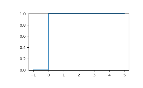
To turn on at t = 1, shift t.
>>> x = step(t - 1.0)
>>> plt.ylim([-0.01, 1.01])
>>> plt.plot(t,x)
-
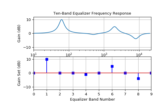
sk_dsp_comm.sigsys.ten_band_eq_filt(x, GdB, Q=3.5)[source]¶ Filter the input signal x with a ten-band equalizer having octave gain values in ndarray GdB.
The signal x is filtered using octave-spaced peaking filters starting at 31.25 Hz and stopping at 16 kHz. The Q of each filter is 3.5, but can be changed. The sampling rate is assumed to be 44.1 kHz.
Parameters: - x : ndarray of the input signal samples
- GdB : ndarray containing ten octave band gain values [G0dB,…,G9dB]
- Q : Quality factor vector for each of the NB peaking filters
Returns: - y : ndarray of output signal samples
Examples
>>> # Test with white noise
>>> w = randn(100000)
>>> y = ten_band_eq_filt(x,GdB)
>>> psd(y,2**10,44.1)
-
sk_dsp_comm.sigsys.ten_band_eq_resp(GdB, Q=3.5)[source]¶ Create a frequency response magnitude plot in dB of a ten band equalizer using a semilogplot (semilogx()) type plot
Parameters: - GdB : Gain vector for 10 peaking filters [G0,…,G9]
- Q : Quality factor for each peaking filter (default 3.5)
Returns: - Nothing : two plots are created
Examples
>>> import matplotlib.pyplot as plt
>>> from sk_dsp_comm import sigsys as ss
>>> ss.ten_band_eq_resp([0,10.0,0,0,-1,0,5,0,-4,0])
>>> plt.show()
-
sk_dsp_comm.sigsys.to_wav(filename, rate, x)[source]¶ Write a wave file.
A wrapper function for scipy.io.wavfile.write that also includes int16 scaling and conversion. Assume input x is [-1,1] values.
Parameters: - filename : file name string
- rate : sampling frequency in Hz
Returns: - Nothing : writes only the *.wav file
Examples
>>> to_wav('test_file.wav', 8000, x)
-
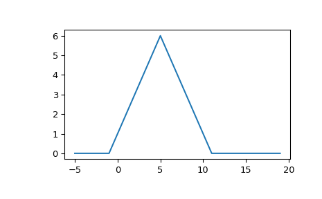
sk_dsp_comm.sigsys.tri(t, tau)[source]¶ Approximation to the triangle pulse Lambda(t/tau).
In this numerical version of Lambda(t/tau) the pulse is active over -tau <= t <= tau.
Parameters: - t : ndarray of the time axis
- tau : one half the triangle base width
Returns: - x : ndarray of the signal Lambda(t/tau)
Examples
>>> import matplotlib.pyplot as plt
>>> from numpy import arange
>>> from sk_dsp_comm.sigsys import tri
>>> t = arange(-1,5,.01)
>>> x = tri(t,1.0)
>>> plt.plot(t,x)
>>> plt.show()
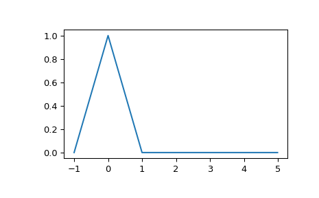
To turn on at t = 1, shift t.
>>> x = tri(t - 1.0,1.0)
>>> plt.plot(t,x)
-
sk_dsp_comm.sigsys.unique_cpx_roots(rlist, tol=0.001)[source]¶ The average of the root values is used when multiplicity is greater than one.
Mark Wickert October 2016
-
sk_dsp_comm.sigsys.upsample(x, L)[source]¶ Upsample by factor L
Insert L - 1 zero samples in between each input sample.
Parameters: - x : ndarray of input signal values
- L : upsample factor
Returns: - y : ndarray of the output signal values
Examples
>>> y = upsample(x,3)
-
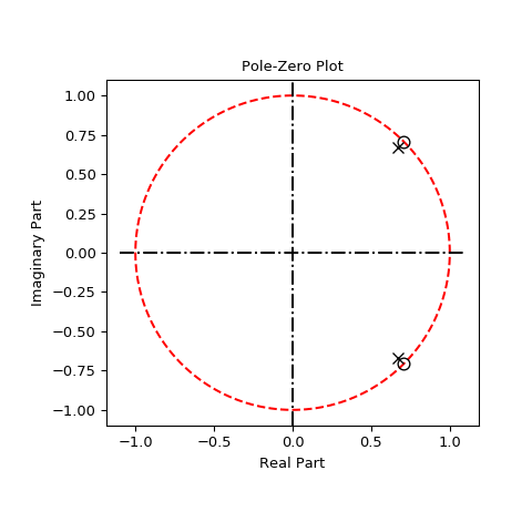
sk_dsp_comm.sigsys.zplane(b, a, auto_scale=True, size=2, detect_mult=True, tol=0.001)[source]¶ Create an z-plane pole-zero plot.
Create an z-plane pole-zero plot using the numerator and denominator z-domain system function coefficient ndarrays b and a respectively. Assume descending powers of z.
Parameters: - b : ndarray of the numerator coefficients
- a : ndarray of the denominator coefficients
- auto_scale : bool (default True)
- size : plot radius maximum when scale = False
Returns: - (M,N) : tuple of zero and pole counts + plot window
Notes
This function tries to identify repeated poles and zeros and will place the multiplicity number above and to the right of the pole or zero. The difficulty is setting the tolerance for this detection. Currently it is set at 1e-3 via the function signal.unique_roots.
Examples
>>> # Here the plot is generated using auto_scale
>>> zplane(b,a)
>>> # Here the plot is generated using manual scaling
>>> zplane(b,a,False,1.5)