%pylab inline
import sk_dsp_comm.sigsys as ss
import sk_dsp_comm.fir_design_helper as fir_d
import sk_dsp_comm.iir_design_helper as iir_d
import sk_dsp_comm.multirate_helper as mrh
import scipy.signal as signal
from IPython.display import Audio, display
from IPython.display import Image, SVG

%pylab is deprecated, use %matplotlib inline and import the required libraries.
Populating the interactive namespace from numpy and matplotlib

%config InlineBackend.figure_formats=['svg'] # SVG inline viewing

Filter Design Using the Helper Modules

The Scipy package signal assists with the design of many digital filter types. As an alternative, here we explore the use of the filter design modules found in scikit-dsp-comm (https://github.com/mwickert/scikit-dsp-comm).

In this note we briefly explore the use of sk_dsp_comm.fir_design_helper and sk_dsp_comm.iir_design_helper. In the examples that follow we assume the import of these modules is made as follows:

import sk_dsp_comm.fir_design_helper as fir_d
import sk_dsp_comm.iir_design_helper as iir_d

The functions in these modules provide an easier and more consistent interface for both finte impulse response (FIR) (linear phase) and infinite impulse response (IIR) classical designs. Functions inside these modules wrap scipy.signal functions and also incorporate new functionality.

Design From Amplitude Response Requirements

With both fir_design_helper and iir_design_helper a design starts with amplitude response requirements, that is the filter passband critical frequencies, stopband critical frequencies, passband ripple, and stopband attenuation. The number of taps/coefficients (FIR case) or the filter order (IIR case) needed to meet these requirements is then determined and the filter coefficients are returned as an ndarray b for FIR, and for IIR both b and a arrays, and a second-order sections sos 2D array, with the rows containing the corresponding cascade of second-order sections toplogy for IIR filters.

For the FIR case we have in the \(z\)-domain

\[H_\text{FIR}(z) = \sum_{k=0}^N b_k z^{-k}\]

with ndarray b = \([b_0, b_1, \ldots, b_N]\). For the IIR case we have in the \(z\)-domain

\[\begin{split}\begin{align} H_\text{IIR}(z) &= \frac{\sum_{k=0}^M b_k z^{-k}}{\sum_{k=1}^N a_k z^{-k}} \\ &= \prod_{k=0}^{N_s-1} \frac{b_{k0} + b_{k1} z^{-1} + b_{k2} z^{-2}}{1 + a_{k1} z^{-1} + a_{k2} z^{-2}} = \prod_{k=0}^{N_s-1} H_k(z) \end{align}\end{split}\]

where \(N_s = \lfloor(N+1)/2\rfloor\). For the b/a form the coefficients are arranged as

b = [b0, b1, ..., bM-1], the numerator filter coefficients
a = [a0, a1, ..., aN-1], the denominator filter ceofficients

For the sos form each row of the 2D sos array corresponds to the coefficients of \(H_k(z)\), as follows:

SOS_mat = [[b00, b01, b02, 1, a01, a02], #biquad 0
           [b10, b11, b12, 1, a11, a12], #biquad 1
            .
            .
           [bNs-10, bNs-11, bNs-12, 1, aNs-11, aNs-12]] #biquad Ns-1

Linear Phase FIR Filter Design

The primary focus of this module is adding the ability to design linear phase FIR filters from user friendly amplitude response requirements.

Most digital filter design is motivated by the desire to approach an ideal filter. Recall an ideal filter will pass signals of a certain of frequencies and block others. For both analog and digital filters the designer can choose from a variety of approximation techniques. For digital filters the approximation techniques fall into the categories of IIR or FIR. In the design of FIR filters two popular techniques are truncating the ideal filter impulse response and applying a window, and optimum equiripple approximations Oppenheim2010. Frequency sampling based approaches are also popular, but will not be considered here, even though scipy.signal supports all three. 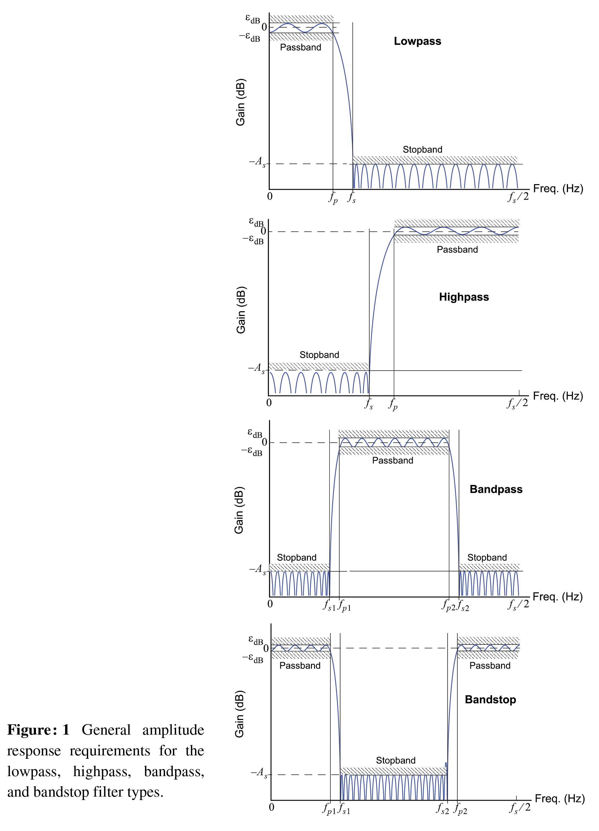Filter design generally begins with a specification of the desired frequency response. The filter frequency response may be stated in several ways, but amplitude response is the most common, e.g., state how \(H_c(j\Omega)\) or \(H(e^{j\omega}) = H(e^{j2\pi f/f_s})\) should behave. A completed design consists of the number of coefficients (taps) required and the coefficients themselves (double precision float or float64 in Numpy, and float64_t in C). Figure 1, below, shows amplitude response requirements in terms of filter gain and critical frequencies for lowpass, highpass, bandpass, and bandstop filters. The critical frequencies are given here in terms of analog requirements in Hz. The sampling frequency is assumed to be in Hz. The passband ripple and stopband attenuation values are in dB. Note in dB terms attenuation is the negative of gain, e.g., -60 of stopband gain is equivalent to 60 dB of stopband attenuation.

Image('300ppi/FIR_Lowpass_Highpass_Bandpass_Bandstop@300ppi.png',width='90%')

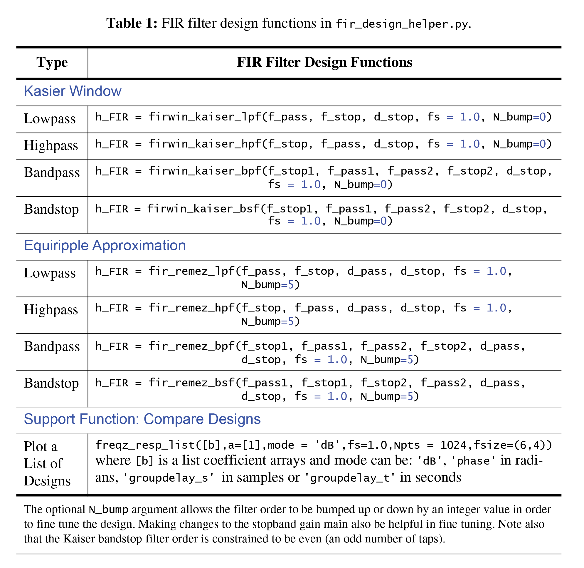
There are 10 filter design functions and one plotting function available in fir_design_helper.py. Four functions for designing Kaiser window based FIR filters and four functions for designing equiripple based FIR filters. Of the eight just described, they all take in amplitude response requirements and return a coefficients array. Two of the 10 filter functions are simply wrappers around the scipy.signal function signal.firwin() for designing filters of a specific order when one (lowpass) or two (bandpass) critical frequencies are given. The wrapper functions fix the window type to the firwin default of hann (hanning). The remamining eight are described below in Table 1. The plotting function provides an easy means to compare the resulting frequency response of one or more designs on a single plot. Display modes allow gain in dB, phase in radians, group delay in samples, and group delay in seconds for a given sampling rate. This function, freq_resp_list(), works for both FIR and IIR designs. Table 1 provides the interface details to the eight design functions where d_stop and d_pass are positive dB values and the critical frequencies have the same unit as the sampling frequency \(f_s\). These functions do not create perfect results so some tuning of of the design parameters may be needed, in addition to bumping the filter order up or down via N_bump.

Image('300ppi/FIR_Kaiser_Equiripple_Table@300ppi.png',width='80%')

Design Examples

Example 1: Lowpass with \(f_s = 1\) Hz

For this 31 tap filter we choose the cutoff frequency to be \(F_c = F_s/8\), or in normalized form \(f_c = 1/8\).

b_k = fir_d.firwin_kaiser_lpf(1/8,1/6,50,1.0)
b_r = fir_d.fir_remez_lpf(1/8,1/6,0.2,50,1.0)

fir_d.freqz_resp_list([b_k,b_r],[[1],[1]],'dB',fs=1)
ylim([-80,5])
title(r'Kaiser vs Equal Ripple Lowpass')
ylabel(r'Filter Gain (dB)')
xlabel(r'Frequency in kHz')
legend((r'Kaiser: %d taps' % len(b_k),r'Remez: %d taps' % len(b_r)),loc='best')
grid();

b_k_hp = fir_d.firwin_kaiser_hpf(1/8,1/6,50,1.0)
b_r_hp = fir_d.fir_remez_hpf(1/8,1/6,0.2,50,1.0)

fir_d.freqz_resp_list([b_k_hp,b_r_hp],[[1],[1]],'dB',fs=1)
ylim([-80,5])
title(r'Kaiser vs Equal Ripple Lowpass')
ylabel(r'Filter Gain (dB)')
xlabel(r'Frequency in kHz')
legend((r'Kaiser: %d taps' % len(b_k),r'Remez: %d taps' % len(b_r)),loc='best')
grid();

b_k_bp = fir_d.firwin_kaiser_bpf(7000,8000,14000,15000,50,48000)
b_r_bp = fir_d.fir_remez_bpf(7000,8000,14000,15000,0.2,50,48000)

fir_d.freqz_resp_list([b_k_bp,b_r_bp],[[1],[1]],'dB',fs=48)
ylim([-80,5])
title(r'Kaiser vs Equal Ripple Bandpass')
ylabel(r'Filter Gain (dB)')
xlabel(r'Frequency in kHz')
legend((r'Kaiser: %d taps' % len(b_k_bp),
        r'Remez: %d taps' % len(b_r_bp)),
       loc='lower right')
grid();

A Design Example Useful for Interpolation or Decimation

Here we consider a lowpass design that needs to pass frequencies from [0, 4000] Hz with a sampling rate of 96000 Hz. This scenario arises when building an interpolator using the classes of the scikit-dps-comm module multirate_helper.py to increase the sampling rate from 8000 Hz to 96000 Hz, or an interpolation factor of \(L = 12\). Note at the top of this notebook we have also have the import

import sk_dsp_comm.multirate_helper as mrh

so that some of the functionality can be accessed. For more details on the use of multirate_helper see.

Start with an equalripple design having transition band centered on 4000 Hz with passband ripple of 0.5 dB and stopband attenuation of 60 dB.

b_up = fir_d.fir_remez_lpf(3300,4300,0.5,60,96000)

mr_up = mrh.multirate_FIR(b_up)

• Consider the pole-zero configuration for this high-order filter

# Take a look at the pole-zero configuration of this very
# high-order (many taps) linear phase FIR
mr_up.zplane()

• Check out the passband and stopband gains

# Verify the passband and stopband gains are as expected
mr_up.freq_resp('db',96000)

• See that the group delay is the expected value of \((N_\text{taps} - 1)/2 = 98\) samples

(len(b_up-1))/2

98.0

# Verify that the FIR design has constant group delay (N_taps - 1)/2 samples
mr_up.freq_resp('groupdelay_s',96000,[0,100])

The object mr_up can now be used for interpolation or decimation with a rate change factor of 12.

Traditional IIR Filter Design using the Bilinear Transform

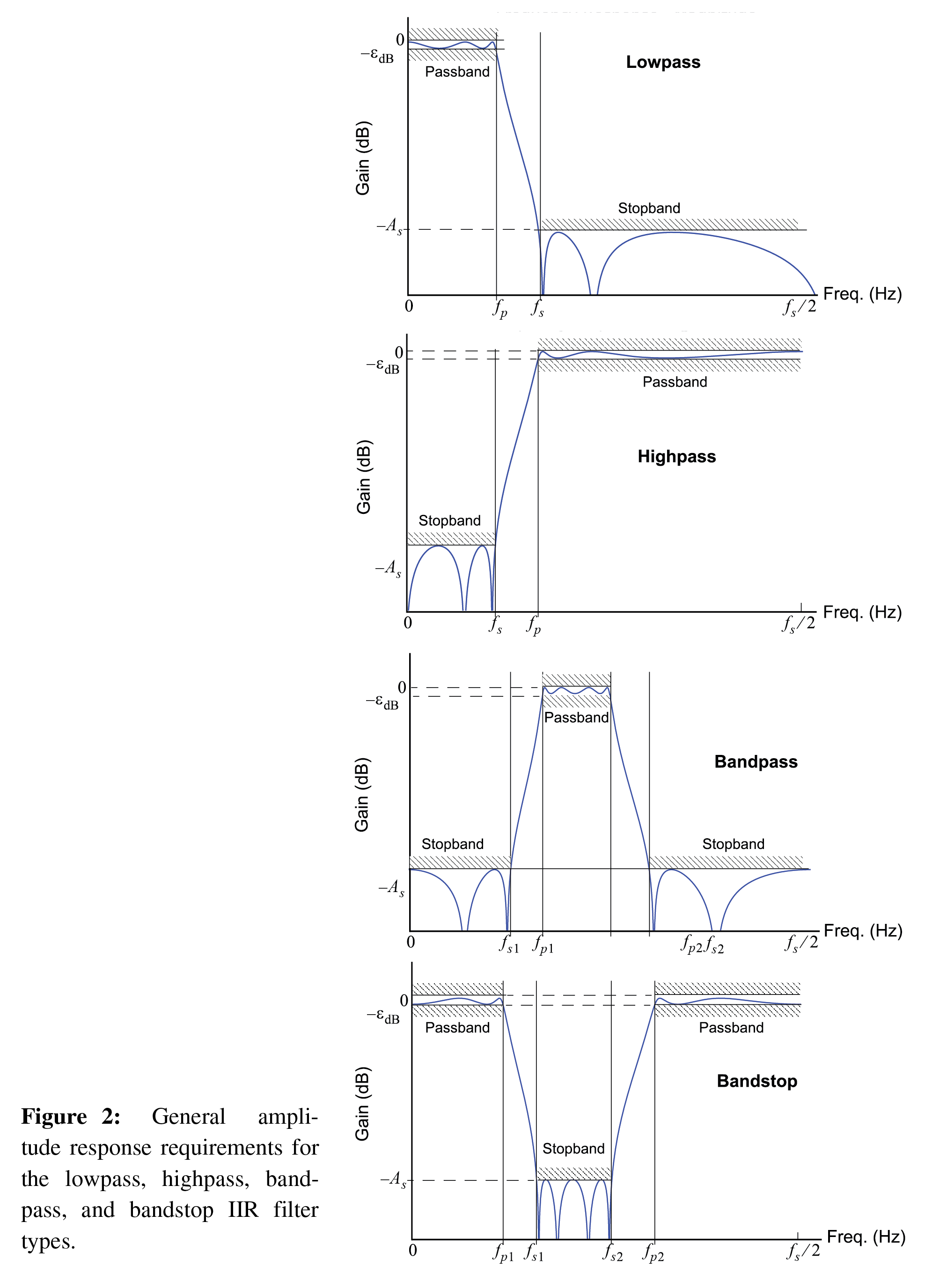
The scipy.signal package fully supports the design of IIR digital filters from analog prototypes. IIR filters like FIR filters, are typically designed with amplitude response requirements in mind. A collection of design functions are available directly from scipy.signal for this purpose, in particular the function scipy.signal.iirdesign(). To make the design of lowpass, highpass, bandpass, and bandstop filters consistent with the module fir_design_helper.py the module iir_design_helper.py was written. Figure 2, below, details how the amplitude response parameters are defined graphically.

Image('300ppi/IIR_Lowpass_Highpass_Bandpass_Bandstop@300ppi.png',width='90%')

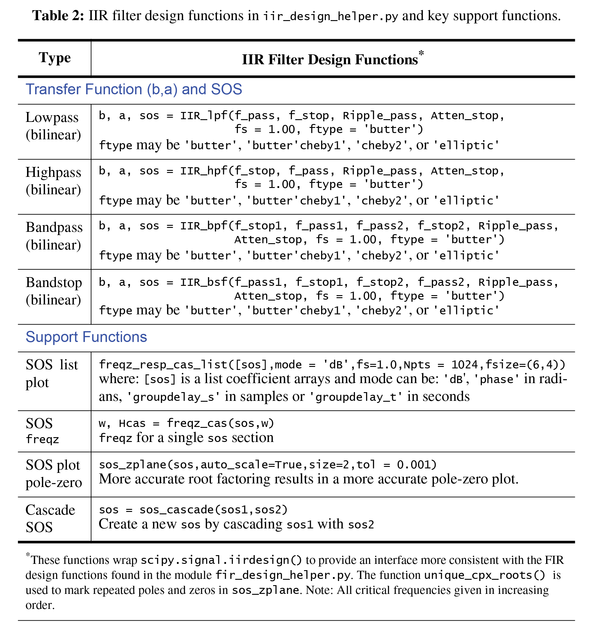
Within iir_design_helper.py there are four filter design functions and a collection of supporting functions available. The four filter design functions are used for designing lowpass, highpass, bandpass, and bandstop filters, utilizing Butterworth, Chebshev type 1, Chebyshev type 2, and elliptical filter prototypes. See Oppenheim2010 and ECE 5650 notes Chapter 9 for detailed design information. The function interfaces are described in Table 2.

Image('300ppi/IIR_Table@300ppi.png',width='80%')

The filter functions return the filter coefficients in two formats:

1. Traditional transfer function form as numerator coefficients b and denominator a coefficients arrays, and

2. Cascade of biquadratic sections form using the previously introduced sos 2D array or matrix.

Both are provided to allow further analysis with either a direct form topology or the sos form. The underlying signal.iirdesign() function also provides a third option: a list of poles and zeros. The sos form desireable for high precision filters, as it is more robust to coefficient quantization, in spite using double precision coefficients in the b and a arrays.

Of the remaining support functions four are also described in Table 2, above. The most significant functions are freqz_resp_cas_list, available for graphically comparing the frequency response over several designs, and sos_zplane a function for plotting the pole-zero pattern. Both operate using the sos matrix. A transfer function form (b/a) for frequency response plotting, freqz_resp_list, is also present in the module. This function was first introduced in the FIR design section. The frequency response function plotting offers modes for gain in dB, phase in radians, group delay in samples, and group delay in seconds, all for a given sampling rate in Hz. The pole-zero plotting function locates pole and zeros more accurately than sk_dsp_commsigsys.zplane, as the numpy function roots() is only solving quadratic polynomials. Also, repeated roots can be displayed as theoretically expected, and also so noted in the graphical display by superscripts next to the pole and zero markers.

IIR Design Based on the Bilinear Transformation

There are multiple ways of designing IIR filters based on amplitude response requirements. When the desire is to have the filter approximation follow an analog prototype such as Butterworth, Chebychev, etc., is using the bilinear transformation. The function signal.iirdesign() described above does exactly this.

In the example below we consider lowpass amplitude response requirements and see how the filter order changes when we choose different analog prototypes.

Example: Lowpass Design Comparison

The lowpass amplitude response requirements given \(f_s = 48\) kHz are: 1. \(f_\text{pass} = 5\) kHz 2. \(f_\text{stop} = 8\) kHz 3. Passband ripple of 0.5 dB 4. Stopband attenuation of 60 dB

Design four filters to meet the same requirements: butter, cheby1, ,cheby2, and ellip:

fs = 48000
f_pass = 5000
f_stop = 8000
b_but,a_but,sos_but = iir_d.IIR_lpf(f_pass,f_stop,0.5,60,fs,'butter')
b_cheb1,a_cheb1,sos_cheb1 = iir_d.IIR_lpf(f_pass,f_stop,0.5,60,fs,'cheby1')
b_cheb2,a_cheb2,sos_cheb2 = iir_d.IIR_lpf(f_pass,f_stop,0.5,60,fs,'cheby2')
b_elli,a_elli,sos_elli = iir_d.IIR_lpf(f_pass,f_stop,0.5,60,fs,'ellip')

Frequency Response Comparison

Here we compare the magnitude response in dB using the sos form of each filter as the input. The elliptic is the most efficient, and actually over achieves by reaching the stopband requirement at less than 8 kHz.

iir_d.freqz_resp_cas_list([sos_but,sos_cheb1,sos_cheb2,sos_elli],'dB',fs=48)
ylim([-80,5])
title(r'IIR Lowpass Compare')
ylabel(r'Filter Gain (dB)')
xlabel(r'Frequency in kHz')
legend((r'Butter order: %d' % (len(a_but)-1),
        r'Cheby1 order: %d' % (len(a_cheb1)-1),
        r'Cheby2 order: %d' % (len(a_cheb2)-1),
        r'Elliptic order: %d' % (len(a_elli)-1)),loc='best')
grid();

Next plot the pole-zero configuration of just the butterworth design. Here we use the a special version of ss.zplane that works with the sos 2D array.

iir_d.sos_zplane(sos_but)

(15, 15)

Note the two plots above can also be obtained using the transfer function form via iir_d.freqz_resp_list([b],[a],'dB',fs=48) and ss.zplane(b,a), respectively. The sos form will yield more accurate results, as it is less sensitive to coefficient quantization. This is particularly true for the pole-zero plot, as rooting a 15th degree polynomial is far more subject to errors than rooting a simple quadratic.

For the 15th-order Butterworth the bilinear transformation maps the expected 15 s-domain zeros at infinity to \(z=-1\). If you use sk_dsp_comm.sigsys.zplane() you will find that the 15 zeros at are in a tight circle around \(z=-1\), indicating polynomial rooting errors. Likewise the frequency response will be more accurate.

Signal filtering of ndarray x is done using the filter designs is done using functions from scipy.signal:

1. For transfer function form y = signal.lfilter(b,a,x)

2. For sos form y = signal.sosfilt(sos,x)

A Half-Band Filter Design to Pass up to \(W/2\) when \(f_s = 8\) kHz

Here we consider a lowpass design that needs to pass frequencies up to \(f_s/4\). Specifically when \(f_s = 8000\) Hz, the filter passband becomes [0, 2000] Hz. Once the coefficients are found a mrh.multirate object is created to allow further study of the filter, and ultimately implement filtering of a white noise signal.

Start with an elliptical design having transition band centered on 2000 Hz with passband ripple of 0.5 dB and stopband attenuation of 80 dB. The transition bandwidth is set to 100 Hz, with 50 Hz on either side of 2000 Hz.

# Elliptic IIR Lowpass
b_lp,a_lp,sos_lp = iir_d.IIR_lpf(1950,2050,0.5,80,8000.,'ellip')
mr_lp = mrh.multirate_IIR(sos_lp)

mr_lp.freq_resp('db',8000)

Pass Gaussian white noise of variance \(\sigma_x^2 = 1\) through the filter. Use a lot of samples so the spectral estimate can accurately form \(S_y(f) = \sigma_x^2\cdot |H(e^{j2\pi f/f_s})|^2 = |H(e^{j2\pi f/f_s})|^2\).

x = randn(1000000)
y = mr_lp.filter(x)
psd(x,2**10,8000);
psd(y,2**10,8000);
title(r'Filtering White Noise Having $\sigma_x^2 = 1$')
legend(('Input PSD','Output PSD'),loc='best')
ylim([-130,-30])

(-130.0, -30.0)

fs = 8000
print('Expected PSD of %2.3f dB/Hz' % (0-10*log10(fs),))

Expected PSD of -39.031 dB/Hz

Amplitude Response Bandpass Design

Here we consider FIR and IIR bandpass designs for use in an SSB demodulator to remove potential adjacent channel signals sitting either side of a frequency band running from 23 kHz to 24 kHz.

b_rec_bpf1 = fir_d.fir_remez_bpf(23000,24000,28000,29000,0.5,70,96000,8)
fir_d.freqz_resp_list([b_rec_bpf1],[1],mode='dB',fs=96000)
ylim([-80, 5])
grid();

The group delay is flat (constant) by virture of the design having linear phase.

b_rec_bpf1 = fir_d.fir_remez_bpf(23000,24000,28000,29000,0.5,70,96000,8)
fir_d.freqz_resp_list([b_rec_bpf1],[1],mode='groupdelay_s',fs=96000)
grid();

Compare the FIR design with an elliptical design:

b_rec_bpf2,a_rec_bpf2,sos_rec_bpf2 = iir_d.IIR_bpf(23000,24000,28000,29000,
                                                   0.5,70,96000,'ellip')
with np.errstate(divide='ignore'):
    iir_d.freqz_resp_cas_list([sos_rec_bpf2],mode='dB',fs=96000)
ylim([-80, 5])
grid();

This high order elliptic has a nice tight amplitude response for minimal coefficients, but the group delay is terrible:

with np.errstate(divide='ignore', invalid='ignore'): #manage singularity warnings
    iir_d.freqz_resp_cas_list([sos_rec_bpf2],mode='groupdelay_s',fs=96000)
#ylim([-80, 5])
grid();