digitalcom

Digital Communications Function Module

Copyright (c) March 2017, Mark Wickert All rights reserved.

Redistribution and use in source and binary forms, with or without modification, are permitted provided that the following conditions are met:

1. Redistributions of source code must retain the above copyright notice, this list of conditions and the following disclaimer.
2. Redistributions in binary form must reproduce the above copyright notice, this list of conditions and the following disclaimer in the documentation and/or other materials provided with the distribution.

THIS SOFTWARE IS PROVIDED BY THE COPYRIGHT HOLDERS AND CONTRIBUTORS “AS IS” AND ANY EXPRESS OR IMPLIED WARRANTIES, INCLUDING, BUT NOT LIMITED TO, THE IMPLIED WARRANTIES OF MERCHANTABILITY AND FITNESS FOR A PARTICULAR PURPOSE ARE DISCLAIMED. IN NO EVENT SHALL THE COPYRIGHT OWNER OR CONTRIBUTORS BE LIABLE FOR ANY DIRECT, INDIRECT, INCIDENTAL, SPECIAL, EXEMPLARY, OR CONSEQUENTIAL DAMAGES (INCLUDING, BUT NOT LIMITED TO, PROCUREMENT OF SUBSTITUTE GOODS OR SERVICES; LOSS OF USE, DATA, OR PROFITS; OR BUSINESS INTERRUPTION) HOWEVER CAUSED AND ON ANY THEORY OF LIABILITY, WHETHER IN CONTRACT, STRICT LIABILITY, OR TORT (INCLUDING NEGLIGENCE OR OTHERWISE) ARISING IN ANY WAY OUT OF THE USE OF THIS SOFTWARE, EVEN IF ADVISED OF THE POSSIBILITY OF SUCH DAMAGE.

The views and conclusions contained in the software and documentation are those of the authors and should not be interpreted as representing official policies, either expressed or implied, of the FreeBSD Project.

sk_dsp_comm.digitalcom.AWGN_chan(x_bits, EBN0_dB)

Parameters:

x_bits : serial bit stream of 0/1 values.

EBN0_dB : Energy per bit to noise power density ratio in dB of the serial bit stream sent through the AWGN channel. Frequently we equate EBN0 to SNR in link budget calculations.

Returns:

y_bits : Received serial bit stream following hard decisions. This bit will have bit errors. To check the estimated bit error probability use BPSK_BEP() or simply:

>>> Pe_est = sum(xor(x_bits,y_bits))/length(x_bits);
    ..

Mark Wickert, March 2015

sk_dsp_comm.digitalcom.BPSK_BEP(tx_data, rx_data, Ncorr=1024, Ntransient=0)

Count bit errors between a transmitted and received BPSK signal. Time delay between streams is detected as well as ambiquity resolution due to carrier phase lock offsets of \(k*\pi\), k=0,1. The ndarray tx_data is Tx +/-1 symbols as real numbers I. The ndarray rx_data is Rx +/-1 symbols as real numbers I. Note: Ncorr needs to be even

sk_dsp_comm.digitalcom.BPSK_tx(N_bits, Ns, ach_fc=2.0, ach_lvl_dB=-100, pulse='rect', alpha=0.25, M=6)

Generates biphase shift keyed (BPSK) transmitter with adjacent channel interference.

Generates three BPSK signals with rectangular or square root raised cosine (SRC) pulse shaping of duration N_bits and Ns samples per bit. The desired signal is centered on f = 0, which the adjacent channel signals to the left and right are also generated at dB level relative to the desired signal. Used in the digital communications Case Study supplement.

Parameters:

N_bits : the number of bits to simulate

Ns : the number of samples per bit

ach_fc : the frequency offset of the adjacent channel signals (default 2.0)

ach_lvl_dB : the level of the adjacent channel signals in dB (default -100)

pulse : the pulse shape ‘rect’ or ‘src’

alpha : square root raised cosine pulse shape factor (default = 0.25)

M : square root raised cosine pulse truncation factor (default = 6)

Returns:

x : ndarray of the composite signal x0 + ach_lvl*(x1p + x1m)

b : the transmit pulse shape

data0 : the data bits used to form the desired signal; used for error checking

Examples

>>> x,b,data0 = BPSK_tx(1000,10,'src')

sk_dsp_comm.digitalcom.GMSK_bb(N_bits, Ns, MSK=0, BT=0.35)

MSK/GMSK Complex Baseband Modulation x,data = gmsk(N_bits, Ns, BT = 0.35, MSK = 0)

Parameters:

N_bits : number of symbols processed

Ns : the number of samples per bit

MSK : 0 for no shaping which is standard MSK, MSK <> 0 –> GMSK is generated.

BT : premodulation Bb*T product which sets the bandwidth of the Gaussian lowpass filter

Mark Wickert Python version November 2014

sk_dsp_comm.digitalcom.MPSK_BEP_thy(SNR_dB, M, EbN0_Mode=True)

Approximate the bit error probability of MPSK assuming Gray encoding

Mark Wickert November 2018

sk_dsp_comm.digitalcom.MPSK_bb(N_symb, Ns, M, pulse='rect', alpha=0.25, MM=6)

Generate a complex baseband MPSK signal with pulse shaping.

Parameters:

N_symb : number of MPSK symbols to produce

Ns : the number of samples per bit,

M : MPSK modulation order, e.g., 4, 8, 16, …

pulse_type : ‘rect’ , ‘rc’, ‘src’ (default ‘rect’)

alpha : excess bandwidth factor(default 0.25)

MM : single sided pulse duration (default = 6)

Returns:

x : ndarray of the MPSK signal values

b : ndarray of the pulse shape

data : ndarray of the underlying data bits

Notes

Pulse shapes include ‘rect’ (rectangular), ‘rc’ (raised cosine), ‘src’ (root raised cosine). The actual pulse length is 2*M+1 samples. This function is used by BPSK_tx in the Case Study article.

Examples

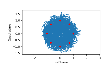
>>> from sk_dsp_comm import digitalcom as dc
>>> import scipy.signal as signal
>>> import matplotlib.pyplot as plt
>>> x,b,data = dc.MPSK_bb(500,10,8,'src',0.35)
>>> # Matched filter received signal x
>>> y = signal.lfilter(b,1,x)
>>> plt.plot(y.real[12*10:],y.imag[12*10:])
>>> plt.xlabel('In-Phase')
>>> plt.ylabel('Quadrature')
>>> plt.axis('equal')
>>> # Sample once per symbol
>>> plt.plot(y.real[12*10::10],y.imag[12*10::10],'r.')
>>> plt.show()

(Source code)

sk_dsp_comm.digitalcom.MPSK_gray_decode(x_hat, M=4)

Decode MPSK IQ symbols to a serial bit stream using gray2bin decoding

x_hat = symbol spaced samples of the MPSK waveform taken at the maximum

eye opening. Normally this is following the matched filter

Mark Wickert November 2018

sk_dsp_comm.digitalcom.MPSK_gray_encode_bb(N_symb, Ns, M=4, pulse='rect', alpha=0.35, M_span=6, ext_data=None)

MPSK_gray_bb: A gray code mapped MPSK complex baseband transmitter x,b,tx_data = MPSK_gray_bb(K,Ns,M)

//////////// Inputs //////////////////////////////////////////////////

N_symb = the number of symbols to process

Ns = number of samples per symbol

M = modulation order: 2, 4, 8, 16 MPSK

alpha = squareroot raised cosine excess bandwidth factor.

Can range over 0 < alpha < 1.

pulse = ‘rect’, ‘src’, or ‘rc’

//////////// Outputs /////////////////////////////////////////////////

x = complex baseband digital modulation b = transmitter shaping filter, rectangle or SRC

tx_data = xI+1j*xQ = inphase symbol sequence +

1j*quadrature symbol sequence

Mark Wickert November 2018

sk_dsp_comm.digitalcom.OFDM_rx(x, Nf, N, Np=0, cp=False, Ncp=0, alpha=0.95, ht=None)

Parameters:

x : Received complex baseband OFDM signal

Nf : Number of filled carriers, must be even and Nf < N

N : Total number of carriers; generally a power 2, e.g., 64, 1024, etc

Np : Period of pilot code blocks; 0 <=> no pilots; -1 <=> use the ht impulse response input to equalize the OFDM symbols; note equalization still requires Ncp > 0 to work on a delay spread channel.

cp : False/True <=> if False assume no CP is present

Ncp : The length of the cyclic prefix

alpha : The filter forgetting factor in the channel estimator. Typically alpha is 0.9 to 0.99.

nt : Input the known theoretical channel impulse response

Returns:

z_out : Recovered complex baseband QAM symbols as a serial stream; as appropriate channel estimation has been applied.

H : channel estimate (in the frequency domain at each subcarrier)

See also

OFDM_tx

Examples

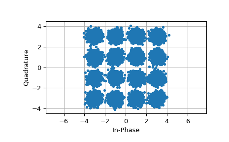
>>> import matplotlib.pyplot as plt
>>> from sk_dsp_comm import digitalcom as dc
>>> from scipy import signal
>>> from numpy import array
>>> hc = array([1.0, 0.1, -0.05, 0.15, 0.2, 0.05]) # impulse response spanning five symbols
>>> # Quick example using the above channel with no cyclic prefix
>>> x1,b1,IQ_data1 = dc.QAM_bb(50000,1,'16qam')
>>> x_out = dc.OFDM_tx(IQ_data1,32,64,0,True,0)
>>> c_out = signal.lfilter(hc,1,x_out) # Apply channel distortion
>>> r_out = dc.cpx_AWGN(c_out,100,64/32) # Es/N0 = 100 dB
>>> z_out,H = dc.OFDM_rx(r_out,32,64,-1,True,0,alpha=0.95,ht=hc)
>>> plt.plot(z_out[200:].real,z_out[200:].imag,'.')
>>> plt.xlabel('In-Phase')
>>> plt.ylabel('Quadrature')
>>> plt.axis('equal')
>>> plt.grid()
>>> plt.show()

(Source code)

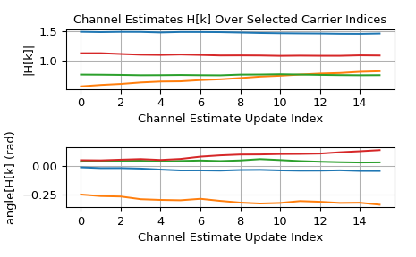
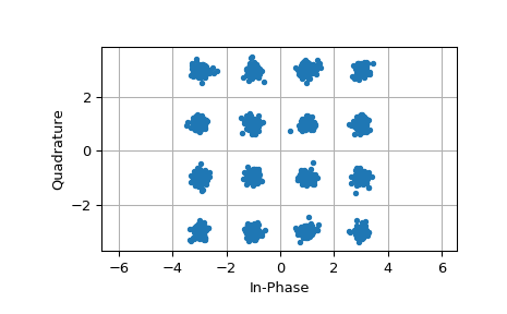
Another example with noise using a 10 symbol cyclic prefix and channel estimation:

>>> x_out = dc.OFDM_tx(IQ_data1,32,64,100,True,10)
>>> c_out = signal.lfilter(hc,1,x_out) # Apply channel distortion
>>> r_out = dc.cpx_AWGN(c_out,25,64/32) # Es/N0 = 25 dB
>>> z_out,H = dc.OFDM_rx(r_out,32,64,100,True,10,alpha=0.95,ht=hc);
>>> plt.figure() # if channel estimation is turned on need this
>>> plt.plot(z_out[-2000:].real,z_out[-2000:].imag,'.') # allow settling time
>>> plt.xlabel('In-Phase')
>>> plt.ylabel('Quadrature')
>>> plt.axis('equal')
>>> plt.grid()
>>> plt.show()

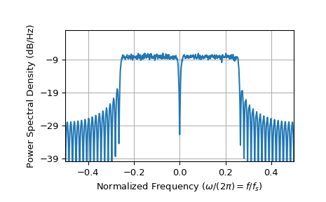
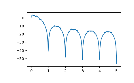
sk_dsp_comm.digitalcom.OFDM_tx(IQ_data, Nf, N, Np=0, cp=False, Ncp=0)

Parameters:

IQ_data : +/-1, +/-3, etc complex QAM symbol sample inputs

Nf : number of filled carriers, must be even and Nf < N

N : total number of carriers; generally a power 2, e.g., 64, 1024, etc

Np : Period of pilot code blocks; 0 <=> no pilots

cp : False/True <=> bypass cp insertion entirely if False

Ncp : the length of the cyclic prefix

Returns:

x_out : complex baseband OFDM waveform output after P/S and CP insertion

See also

OFDM_rx

Examples

>>> import matplotlib.pyplot as plt
>>> from sk_dsp_comm import digitalcom as dc
>>> x1,b1,IQ_data1 = dc.QAM_bb(50000,1,'16qam')
>>> x_out = dc.OFDM_tx(IQ_data1,32,64)
>>> plt.psd(x_out,2**10,1);
>>> plt.xlabel(r'Normalized Frequency ($\omega/(2\pi)=f/f_s$)')
>>> plt.ylim([-40,0])
>>> plt.xlim([-.5,.5])
>>> plt.show()

(Source code)

sk_dsp_comm.digitalcom.PCM_decode(x_bits, N_bits)

Parameters:

x_bits : serial bit stream of 0/1 values. The length of

x_bits must be a multiple of N_bits

N_bits : bit precision of PCM samples

Returns:

xhat : decoded PCM signal samples

Mark Wickert, March 2015

sk_dsp_comm.digitalcom.PCM_encode(x, N_bits)

Parameters:

x : signal samples to be PCM encoded

N_bits ; bit precision of PCM samples

Returns:

x_bits = encoded serial bit stream of 0/1 values. MSB first.

Mark Wickert, Mark 2015

sk_dsp_comm.digitalcom.QAM_BEP_thy(SNR_dB, M, EbN0_Mode=True)

Approximate the bit error probability of QAM assuming Gray encoding

Mark Wickert November 2018

sk_dsp_comm.digitalcom.QAM_SEP(tx_data, rx_data, mod_type, Ncorr = 1024, Ntransient = 0)

Count symbol errors between a transmitted and received QAM signal. The received symbols are assumed to be soft values on a unit square. Time delay between streams is detected. The ndarray tx_data is Tx complex symbols. The ndarray rx_data is Rx complex symbols. Note: Ncorr needs to be even

sk_dsp_comm.digitalcom.QAM_bb(N_symb, Ns, mod_type='16qam', pulse='rect', alpha=0.35)

QAM_BB_TX: A complex baseband transmitter x,b,tx_data = QAM_bb(K,Ns,M)

//////////// Inputs //////////////////////////////////////////////////

N_symb = the number of symbols to process

Ns = number of samples per symbol

mod_type = modulation type: qpsk, 16qam, 64qam, or 256qam

alpha = squareroot raised codine pulse shape bandwidth factor.

For DOCSIS alpha = 0.12 to 0.18. In general alpha can range over 0 < alpha < 1.

SRC = pulse shape: 0-> rect, 1-> SRC

//////////// Outputs /////////////////////////////////////////////////

x = complex baseband digital modulation b = transmitter shaping filter, rectangle or SRC

tx_data = xI+1j*xQ = inphase symbol sequence +

1j*quadrature symbol sequence

Mark Wickert November 2014

sk_dsp_comm.digitalcom.QAM_gray_decode(x_hat, M=4)

Decode MQAM IQ symbols to a serial bit stream using gray2bin decoding

x_hat = symbol spaced samples of the QAM waveform taken at the maximum

eye opening. Normally this is following the matched filter

Mark Wickert April 2018

sk_dsp_comm.digitalcom.QAM_gray_encode_bb(N_symb, Ns, M=4, pulse='rect', alpha=0.35, M_span=6, ext_data=None)

QAM_gray_bb: A gray code mapped QAM complex baseband transmitter x,b,tx_data = QAM_gray_bb(K,Ns,M)

Parameters:

N_symb : The number of symbols to process

Ns : Number of samples per symbol

M : Modulation order: 2, 4, 16, 64, 256 QAM. Note 2 <=> BPSK, 4 <=> QPSK

alpha : Square root raised cosine excess bandwidth factor.

For DOCSIS alpha = 0.12 to 0.18. In general alpha can range over 0 < alpha < 1.

pulse : ‘rect’, ‘src’, or ‘rc’

Returns:

x : Complex baseband digital modulation

b : Transmitter shaping filter, rectangle or SRC

tx_data : xI+1j*xQ = inphase symbol sequence + 1j*quadrature symbol sequence

See also

QAM_gray_decode

sk_dsp_comm.digitalcom.QPSK_BEP(tx_data, rx_data, Ncorr=1024, Ntransient=0)

Count bit errors between a transmitted and received QPSK signal. Time delay between streams is detected as well as ambiquity resolution due to carrier phase lock offsets of \(k*\frac{\pi}{4}\), k=0,1,2,3. The ndarray sdata is Tx +/-1 symbols as complex numbers I + j*Q. The ndarray data is Rx +/-1 symbols as complex numbers I + j*Q. Note: Ncorr needs to be even

sk_dsp_comm.digitalcom.QPSK_bb(N_symb, Ns, lfsr_len=5, pulse='src', alpha=0.25, M=6)

sk_dsp_comm.digitalcom.QPSK_rx(fc, N_symb, Rs, EsN0=100, fs=125, lfsr_len=10, phase=0, pulse='src')

This function generates

sk_dsp_comm.digitalcom.QPSK_tx(fc, N_symb, Rs, fs=125, lfsr_len=10, pulse='src')

sk_dsp_comm.digitalcom.Q_fctn(x)

Gaussian Q-function

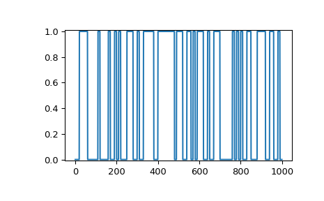
sk_dsp_comm.digitalcom.RZ_bits(N_bits, Ns, pulse='rect', alpha=0.25, M=6)

Generate return-to-zero (RZ) data bits with pulse shaping.

A baseband digital data signal using +/-1 amplitude signal values and including pulse shaping.

Parameters:

N_bits : number of RZ {0,1} data bits to produce

Ns : the number of samples per bit,

pulse_type : ‘rect’ , ‘rc’, ‘src’ (default ‘rect’)

alpha : excess bandwidth factor(default 0.25)

M : single sided pulse duration (default = 6)

Returns:

x : ndarray of the RZ signal values

b : ndarray of the pulse shape

data : ndarray of the underlying data bits

Notes

Pulse shapes include ‘rect’ (rectangular), ‘rc’ (raised cosine), ‘src’ (root raised cosine). The actual pulse length is 2*M+1 samples. This function is used by BPSK_tx in the Case Study article.

Examples

>>> import matplotlib.pyplot as plt
>>> from numpy import arange
>>> from sk_dsp_comm.digitalcom import RZ_bits
>>> x,b,data = RZ_bits(100,10)
>>> t = arange(len(x))
>>> plt.plot(t,x)
>>> plt.ylim([-0.01, 1.01])
>>> plt.show()

(Source code)

sk_dsp_comm.digitalcom.bin2gray(d_word, b_width)

Convert integer bit words to gray encoded binary words via Gray coding starting from the MSB to the LSB

Mark Wickert November 2018

sk_dsp_comm.digitalcom.bit_errors(tx_data, rx_data, Ncorr=1024, Ntransient=0)

Count bit errors between a transmitted and received BPSK signal. Time delay between streams is detected as well as ambiquity resolution due to carrier phase lock offsets of \(k*\pi\), k=0,1. The ndarray tx_data is Tx 0/1 bits as real numbers I. The ndarray rx_data is Rx 0/1 bits as real numbers I. Note: Ncorr needs to be even

sk_dsp_comm.digitalcom.chan_est_equalize(z, Np, alpha, Ht=None)

This is a helper function for OFDM_rx() to unpack pilot blocks from from the entire set of received OFDM symbols (the Nf of N filled carriers only); then estimate the channel array H recursively, and finally apply H_hat to Y, i.e., X_hat = Y/H_hat carrier-by-carrier. Note if Np = -1, then H_hat = H, the true channel.

Parameters:

z : Input N_OFDM x Nf 2D array containing pilot blocks and OFDM data symbols.

Np : The pilot block period; if -1 use the known channel impulse response input to ht.

alpha : The forgetting factor used to recursively estimate H_hat

Ht : The theoretical channel frquency response to allow ideal equalization provided Ncp is adequate.

Returns:

zz_out : The input z with the pilot blocks removed and one-tap equalization applied to each of the Nf carriers.

H : The channel estimate in the frequency domain; an array of length Nf; will return Ht if provided as an input.

Examples

>>> from sk_dsp_comm.digitalcom import chan_est_equalize
>>> zz_out,H = chan_est_eq(z,Nf,Np,alpha,Ht=None)

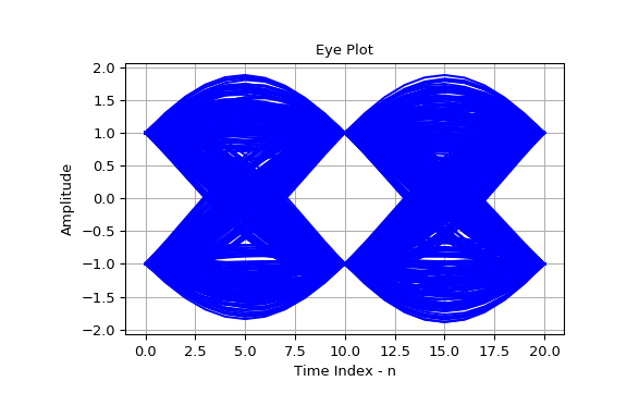
sk_dsp_comm.digitalcom.eye_plot(x, L, S=0)

Eye pattern plot of a baseband digital communications waveform.

The signal must be real, but can be multivalued in terms of the underlying modulation scheme. Used for BPSK eye plots in the Case Study article.

Parameters:

x : ndarray of the real input data vector/array

L : display length in samples (usually two symbols)

S : start index

Returns:

None : A plot window opens containing the eye plot

Notes

Increase S to eliminate filter transients.

Examples

1000 bits at 10 samples per bit with ‘rc’ shaping.

>>> import matplotlib.pyplot as plt
>>> from sk_dsp_comm import digitalcom as dc
>>> x,b, data = dc.NRZ_bits(1000,10,'rc')
>>> dc.eye_plot(x,20,60)
>>> plt.show()

(Source code)

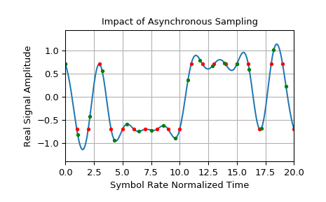
sk_dsp_comm.digitalcom.farrow_resample(x, fs_old, fs_new)

Parameters:

x : Input list representing a signal vector needing resampling.

fs_old : Starting/old sampling frequency.

fs_new : New sampling frequency.

Returns:

y : List representing the signal vector resampled at the new frequency.

Notes

A cubic interpolator using a Farrow structure is used resample the input data at a new sampling rate that may be an irrational multiple of the input sampling rate.

Time alignment can be found for a integer value M, found with the following:

\[f_{s,out} = f_{s,in} (M - 1) / M\]

The filter coefficients used here and a more comprehensive listing can be found in H. Meyr, M. Moeneclaey, & S. Fechtel, “Digital Communication Receivers,” Wiley, 1998, Chapter 9, pp. 521-523.

Another good paper on variable interpolators is: L. Erup, F. Gardner, & R. Harris, “Interpolation in Digital Modems–Part II: Implementation and Performance,” IEEE Comm. Trans., June 1993, pp. 998-1008.

A founding paper on the subject of interpolators is: C. W. Farrow, “A Continuously variable Digital Delay Element,” Proceedings of the IEEE Intern. Symp. on Circuits Syst., pp. 2641-2645, June 1988.

Mark Wickert April 2003, recoded to Python November 2013

Examples

The following example uses a QPSK signal with rc pulse shaping, and time alignment at M = 15.

>>> import matplotlib.pyplot as plt
>>> from numpy import arange
>>> from sk_dsp_comm import digitalcom as dc
>>> Ns = 8
>>> Rs = 1.
>>> fsin = Ns*Rs
>>> Tsin = 1 / fsin
>>> N = 200
>>> ts = 1
>>> x, b, data = dc.MPSK_bb(N+12, Ns, 4, 'rc')
>>> x = x[12*Ns:]
>>> xxI = x.real
>>> M = 15
>>> fsout = fsin * (M-1) / M
>>> Tsout = 1. / fsout
>>> xI = dc.farrow_resample(xxI, fsin, fsin)
>>> tx = arange(0, len(xI)) / fsin
>>> yI = dc.farrow_resample(xxI, fsin, fsout)
>>> ty = arange(0, len(yI)) / fsout
>>> plt.plot(tx - Tsin, xI)
>>> plt.plot(tx[ts::Ns] - Tsin, xI[ts::Ns], 'r.')
>>> plt.plot(ty[ts::Ns] - Tsout, yI[ts::Ns], 'g.')
>>> plt.title(r'Impact of Asynchronous Sampling')
>>> plt.ylabel(r'Real Signal Amplitude')
>>> plt.xlabel(r'Symbol Rate Normalized Time')
>>> plt.xlim([0, 20])
>>> plt.grid()
>>> plt.show()

(Source code)

sk_dsp_comm.digitalcom.from_bin(bin_array)

Convert binary array back a nonnegative integer. The array length is the bit width. The first input index holds the MSB and the last holds the LSB.

sk_dsp_comm.digitalcom.gray2bin(d_word, b_width)

Convert gray encoded binary words to integer bit words via Gray decoding starting from the MSB to the LSB

Mark Wickert November 2018

sk_dsp_comm.digitalcom.mux_pilot_blocks(IQ_data, Np)

Parameters:

IQ_data : a 2D array of input QAM symbols with the columns

representing the NF carrier frequencies and each row the QAM symbols used to form an OFDM symbol

Np : the period of the pilot blocks; e.g., a pilot block is

inserted every Np OFDM symbols (Np-1 OFDM data symbols of width Nf are inserted in between the pilot blocks.

Returns:

IQ_datap : IQ_data with pilot blocks inserted

See also

OFDM_tx

Notes

A helper function called by OFDM_tx() that inserts pilot block for use in channel estimation when a delay spread channel is present.

sk_dsp_comm.digitalcom.my_psd(x, NFFT=1024, Fs=1)

A local version of NumPy’s PSD function that returns the plot arrays.

A mlab.psd wrapper function that returns two ndarrays; makes no attempt to auto plot anything.

Parameters:

x : ndarray input signal

NFFT : a power of two, e.g., 2**10 = 1024

Fs : the sampling rate in Hz

Returns:

Px : ndarray of the power spectrum estimate

f : ndarray of frequency values

Notes

This function makes it easier to overlay spectrum plots because you have better control over the axis scaling than when using psd() in the autoscale mode.

Examples

>>> import matplotlib.pyplot as plt
>>> from sk_dsp_comm import digitalcom as dc
>>> from numpy import log10
>>> x,b, data = dc.NRZ_bits(10000,10)
>>> Px,f = dc.my_psd(x,2**10,10)
>>> plt.plot(f, 10*log10(Px))
>>> plt.show()

(Source code)

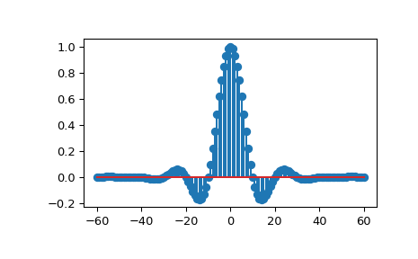
sk_dsp_comm.digitalcom.rc_imp(Ns, alpha, M=6)

A truncated raised cosine pulse used in digital communications.

The pulse shaping factor \(0 < \alpha < 1\) is required as well as the truncation factor M which sets the pulse duration to be \(2*M*T_{symbol}\).

Parameters:

Ns : number of samples per symbol

alpha : excess bandwidth factor on (0, 1), e.g., 0.35

M : equals RC one-sided symbol truncation factor

Returns:

b : ndarray containing the pulse shape

See also

sqrt_rc_imp

Notes

The pulse shape b is typically used as the FIR filter coefficients when forming a pulse shaped digital communications waveform.

Examples

Ten samples per symbol and \(\alpha = 0.35\).

>>> import matplotlib.pyplot as plt
>>> from sk_dsp_comm.digitalcom import rc_imp
>>> from numpy import arange
>>> b = rc_imp(10,0.35)
>>> n = arange(-10*6,10*6+1)
>>> plt.stem(n,b)
>>> plt.show()

(Source code)

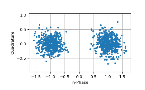
sk_dsp_comm.digitalcom.scatter(x, Ns, start)

Sample a baseband digital communications waveform at the symbol spacing.

Parameters:

x : ndarray of the input digital comm signal

Ns : number of samples per symbol (bit)

start : the array index to start the sampling

Returns:

xI : ndarray of the real part of x following sampling

xQ : ndarray of the imaginary part of x following sampling

Notes

Normally the signal is complex, so the scatter plot contains clusters at point in the complex plane. For a binary signal such as BPSK, the point centers are nominally +/-1 on the real axis. Start is used to eliminate transients from the FIR pulse shaping filters from appearing in the scatter plot.

Examples

>>> import matplotlib.pyplot as plt
>>> from sk_dsp_comm import digitalcom as dc
>>> x,b, data = dc.NRZ_bits(1000,10,'rc')

Add some noise so points are now scattered about +/-1.

>>> y = dc.cpx_AWGN(x,20,10)
>>> yI,yQ = dc.scatter(y,10,60)
>>> plt.plot(yI,yQ,'.')
>>> plt.grid()
>>> plt.xlabel('In-Phase')
>>> plt.ylabel('Quadrature')
>>> plt.axis('equal')
>>> plt.show()

(Source code)

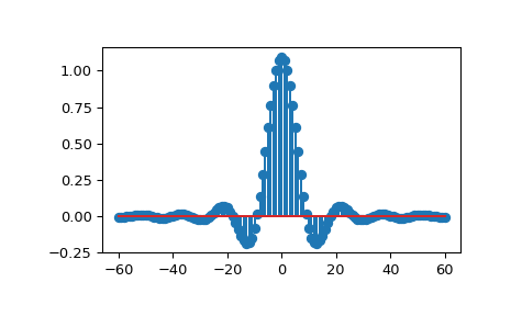
sk_dsp_comm.digitalcom.sqrt_rc_imp(Ns, alpha, M=6)

A truncated square root raised cosine pulse used in digital communications.

The pulse shaping factor \(0 < \alpha < 1\) is required as well as the truncation factor M which sets the pulse duration to be \(2*M*T_{symbol}\).

Parameters:

Ns : number of samples per symbol

alpha : excess bandwidth factor on (0, 1), e.g., 0.35

M : equals RC one-sided symbol truncation factor

Returns:

b : ndarray containing the pulse shape

Notes

The pulse shape b is typically used as the FIR filter coefficients when forming a pulse shaped digital communications waveform. When square root raised cosine (SRC) pulse is used to generate Tx signals and at the receiver used as a matched filter (receiver FIR filter), the received signal is now raised cosine shaped, thus having zero intersymbol interference and the optimum removal of additive white noise if present at the receiver input.

Examples

Ten samples per symbol and \(\alpha = 0.35\).

>>> import matplotlib.pyplot as plt
>>> from numpy import arange
>>> from sk_dsp_comm.digitalcom import sqrt_rc_imp
>>> b = sqrt_rc_imp(10,0.35)
>>> n = arange(-10*6,10*6+1)
>>> plt.stem(n,b)
>>> plt.show()

(Source code)

sk_dsp_comm.digitalcom.strips(x, Nx, fig_size=(6, 4))

Plots the contents of real ndarray x as a vertical stacking of strips, each of length Nx. The default figure size is (6,4) inches. The yaxis tick labels are the starting index of each strip. The red dashed lines correspond to zero amplitude in each strip.

strips(x,Nx,my_figsize=(6,4))

Mark Wickert April 2014

sk_dsp_comm.digitalcom.time_delay(x, D, N=4)

A time varying time delay which takes advantage of the Farrow structure for cubic interpolation:

y = time_delay(x,D,N = 3)

Note that D is an array of the same length as the input signal x. This allows you to make the delay a function of time. If you want a constant delay just use D*zeros(len(x)). The minimum delay allowable is one sample or D = 1.0. This is due to the causal system nature of the Farrow structure.

A founding paper on the subject of interpolators is: C. W. Farrow, “A Continuously variable Digital Delay Element,” Proceedings of the IEEE Intern. Symp. on Circuits Syst., pp. 2641-2645, June 1988.

Mark Wickert, February 2014

sk_dsp_comm.digitalcom.to_bin(data, width)

Convert an unsigned integer to a numpy binary array with the first element the MSB and the last element the LSB.

sk_dsp_comm.digitalcom.xcorr(x1, x2, Nlags)

r12, k = xcorr(x1,x2,Nlags), r12 and k are ndarray’s Compute the energy normalized cross correlation between the sequences x1 and x2. If x1 = x2 the cross correlation is the autocorrelation. The number of lags sets how many lags to return centered about zero