fec_conv
A Convolutional Encoding and Decoding
Copyright (c) March 2017, Mark Wickert All rights reserved.
Redistribution and use in source and binary forms, with or without modification, are permitted provided that the following conditions are met:
Redistributions of source code must retain the above copyright notice, this list of conditions and the following disclaimer.
Redistributions in binary form must reproduce the above copyright notice, this list of conditions and the following disclaimer in the documentation and/or other materials provided with the distribution.
THIS SOFTWARE IS PROVIDED BY THE COPYRIGHT HOLDERS AND CONTRIBUTORS “AS IS” AND ANY EXPRESS OR IMPLIED WARRANTIES, INCLUDING, BUT NOT LIMITED TO, THE IMPLIED WARRANTIES OF MERCHANTABILITY AND FITNESS FOR A PARTICULAR PURPOSE ARE DISCLAIMED. IN NO EVENT SHALL THE COPYRIGHT OWNER OR CONTRIBUTORS BE LIABLE FOR ANY DIRECT, INDIRECT, INCIDENTAL, SPECIAL, EXEMPLARY, OR CONSEQUENTIAL DAMAGES (INCLUDING, BUT NOT LIMITED TO, PROCUREMENT OF SUBSTITUTE GOODS OR SERVICES; LOSS OF USE, DATA, OR PROFITS; OR BUSINESS INTERRUPTION) HOWEVER CAUSED AND ON ANY THEORY OF LIABILITY, WHETHER IN CONTRACT, STRICT LIABILITY, OR TORT (INCLUDING NEGLIGENCE OR OTHERWISE) ARISING IN ANY WAY OUT OF THE USE OF THIS SOFTWARE, EVEN IF ADVISED OF THE POSSIBILITY OF SUCH DAMAGE.
The views and conclusions contained in the software and documentation are those of the authors and should not be interpreted as representing official policies, either expressed or implied, of the FreeBSD Project.
A forward error correcting coding (FEC) class which defines methods for performing convolutional encoding and decoding. Arbitrary polynomials are supported, but the rate is presently limited to r = 1/n, where n = 2. Punctured (perforated) convolutional codes are also supported. The puncturing pattern (matrix) is arbitrary.
Two popular encoder polynomial sets are:
K = 3 ==> G1 = ‘111’, G2 = ‘101’ and K = 7 ==> G1 = ‘1011011’, G2 = ‘1111001’.
A popular puncturing pattern to convert from rate 1/2 to rate 3/4 is a G1 output puncture pattern of ‘110’ and a G2 output puncture pattern of ‘101’.
Graphical display functions are included to allow the user to better understand the operation of the Viterbi decoder.
Mark Wickert and Andrew Smit: October 2018.
- class sk_dsp_comm.fec_conv.FECConv(G=('111', '101'), Depth=10)[source]
Class responsible for creating rate 1/2 convolutional code objects, and then encoding and decoding the user code set in polynomials of G. Key methods provided include
conv_encoder(),viterbi_decoder(),puncture(),depuncture(),trellis_plot(), andtraceback_plot().- Parameters
- G: A tuple of two binary strings corresponding to the encoder polynomials
- Depth: The decision depth employed by the Viterbi decoder method
Examples
>>> from sk_dsp_comm import fec_conv
>>> # Rate 1/2
>>> cc1 = fec_conv.FECConv(('101', '111'), Depth=10)  # decision depth is 10
>>> # Rate 1/3
>>> from sk_dsp_comm import fec_conv
>>> cc2 = fec_conv.FECConv(('101','011','111'), Depth=15)  # decision depth is 15
Methods
bm_calc(ref_code_bits, rec_code_bits, …)distance = bm_calc(ref_code_bits, rec_code_bits, metric_type) Branch metrics calculation
conv_encoder(input, state)output, state = conv_encoder(input,state) We get the 1/2 or 1/3 rate from self.rate Polys G1 and G2 are entered as binary strings, e.g, G1 = ‘111’ and G2 = ‘101’ for K = 3 G1 = ‘1011011’ and G2 = ‘1111001’ for K = 7 G3 is also included for rate 1/3 Input state as a binary string of length K-1, e.g., ‘00’ or ‘0000000’ e.g., state = ‘00’ for K = 3 e.g., state = ‘000000’ for K = 7 Mark Wickert and Andrew Smit 2018
depuncture(soft_bits[, puncture_pattern, …])Apply de-puncturing to the soft bits coming from the channel.
puncture(code_bits[, puncture_pattern])Apply puncturing to the serial bits produced by convolutionally encoding.
traceback_plot([fsize])Plots a path of the possible last 4 states.
trellis_plot([fsize])Plots a trellis diagram of the possible state transitions.
viterbi_decoder(x[, metric_type, quant_level])A method which performs Viterbi decoding of noisy bit stream, taking as input soft bit values centered on +/-1 and returning hard decision 0/1 bits.
- bm_calc(ref_code_bits, rec_code_bits, metric_type, quant_level)[source]
distance = bm_calc(ref_code_bits, rec_code_bits, metric_type) Branch metrics calculation
Mark Wickert and Andrew Smit October 2018
- conv_encoder(input, state)[source]
output, state = conv_encoder(input,state) We get the 1/2 or 1/3 rate from self.rate Polys G1 and G2 are entered as binary strings, e.g, G1 = ‘111’ and G2 = ‘101’ for K = 3 G1 = ‘1011011’ and G2 = ‘1111001’ for K = 7 G3 is also included for rate 1/3 Input state as a binary string of length K-1, e.g., ‘00’ or ‘0000000’ e.g., state = ‘00’ for K = 3 e.g., state = ‘000000’ for K = 7 Mark Wickert and Andrew Smit 2018
- depuncture(soft_bits, puncture_pattern=('110', '101'), erase_value=3.5)[source]
Apply de-puncturing to the soft bits coming from the channel. Erasure bits are inserted to return the soft bit values back to a form that can be Viterbi decoded.
- Parameters
soft_bits –
puncture_pattern –
erase_value –
- Returns
Examples
This example uses the following puncture matrix:
\[\begin{split}\begin{align*} \mathbf{A} = \begin{bmatrix} 1 & 1 & 0 \\ 1 & 0 & 1 \end{bmatrix} \end{align*}\end{split}\]The upper row operates on the outputs for the \(G_{1}\) polynomial and the lower row operates on the outputs of the \(G_{2}\) polynomial.
>>> import numpy as np
>>> from sk_dsp_comm.fec_conv import FECConv
>>> cc = FECConv(('101','111'))
>>> x = np.array([0, 0, 1, 1, 1, 0, 0, 0, 0, 0])
>>> state = '00'
>>> y, state = cc.conv_encoder(x, state)
>>> yp = cc.puncture(y, ('110','101'))
>>> cc.depuncture(yp, ('110', '101'), 1)
array([ 0., 0., 0., 1., 1., 1., 1., 0., 0., 1., 1., 0., 1., 1., 0., 1., 1., 0.]
- puncture(code_bits, puncture_pattern=('110', '101'))[source]
Apply puncturing to the serial bits produced by convolutionally encoding.
- Parameters
code_bits –
puncture_pattern –
- Returns
Examples
This example uses the following puncture matrix:
\[\begin{split}\begin{align*} \mathbf{A} = \begin{bmatrix} 1 & 1 & 0 \\ 1 & 0 & 1 \end{bmatrix} \end{align*}\end{split}\]The upper row operates on the outputs for the \(G_{1}\) polynomial and the lower row operates on the outputs of the \(G_{2}\) polynomial.
>>> import numpy as np
>>> from sk_dsp_comm.fec_conv import FECConv
>>> cc = FECConv(('101','111'))
>>> x = np.array([0, 0, 1, 1, 1, 0, 0, 0, 0, 0])
>>> state = '00'
>>> y, state = cc.conv_encoder(x, state)
>>> cc.puncture(y, ('110','101'))
array([ 0.,  0.,  0.,  1.,  1.,  0.,  0.,  0.,  1.,  1.,  0.,  0.])
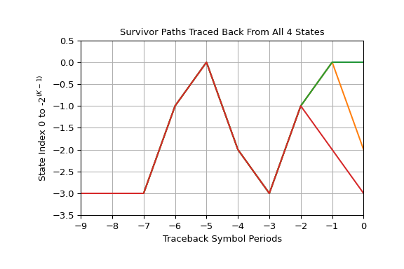
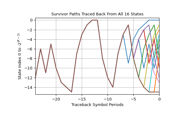
- traceback_plot(fsize=(6, 4))[source]
Plots a path of the possible last 4 states.
- Parameters
- fsizePlot size for matplotlib.
Examples
>>> import matplotlib.pyplot as plt
>>> from sk_dsp_comm.fec_conv import FECConv
>>> from sk_dsp_comm import digitalcom as dc
>>> import numpy as np
>>> cc = FECConv()
>>> x = np.random.randint(0,2,100)
>>> state = '00'
>>> y,state = cc.conv_encoder(x,state)
>>> # Add channel noise to bits translated to +1/-1
>>> yn = dc.cpx_awgn(2*y-1,5,1) # SNR = 5 dB
>>> # Translate noisy +1/-1 bits to soft values on [0,7]
>>> yn = (yn.real+1)/2*7
>>> z = cc.viterbi_decoder(yn)
>>> cc.traceback_plot()
>>> plt.show()
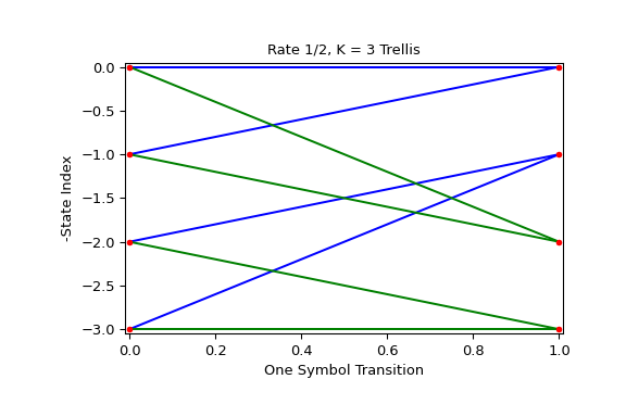
- trellis_plot(fsize=(6, 4))[source]
Plots a trellis diagram of the possible state transitions.
- Parameters
- fsizePlot size for matplotlib.
Examples
>>> import matplotlib.pyplot as plt
>>> from sk_dsp_comm.fec_conv import FECConv
>>> cc = FECConv()
>>> cc.trellis_plot()
>>> plt.show()
- viterbi_decoder(x, metric_type='soft', quant_level=3)[source]
A method which performs Viterbi decoding of noisy bit stream, taking as input soft bit values centered on +/-1 and returning hard decision 0/1 bits.
- Parameters
- x: Received noisy bit values centered on +/-1 at one sample per bit
- metric_type:
‘hard’ - Hard decision metric. Expects binary or 0/1 input values. ‘unquant’ - unquantized soft decision decoding. Expects +/-1
input values.
‘soft’ - soft decision decoding.
- quant_level: The quantization level for soft decoding. Expected
- input values between 0 and 2^quant_level-1. 0 represents the most
- confident 0 and 2^quant_level-1 represents the most confident 1.
- Only used for ‘soft’ metric type.
- Returns
- y: Decoded 0/1 bit stream
Examples
>>> import numpy as np
>>> from numpy.random import randint
>>> import sk_dsp_comm.fec_conv as fec
>>> import sk_dsp_comm.digitalcom as dc
>>> import matplotlib.pyplot as plt
>>> # Soft decision rate 1/2 simulation
>>> N_bits_per_frame = 10000
>>> EbN0 = 4
>>> total_bit_errors = 0
>>> total_bit_count = 0
>>> cc1 = fec.FECConv(('11101','10011'),25)
>>> # Encode with shift register starting state of '0000'
>>> state = '0000'
>>> while total_bit_errors < 100:
>>>     # Create 100000 random 0/1 bits
>>>     x = randint(0,2,N_bits_per_frame)
>>>     y,state = cc1.conv_encoder(x,state)
>>>     # Add channel noise to bits, include antipodal level shift to [-1,1]
>>>     yn_soft = dc.cpx_awgn(2*y-1,EbN0-3,1) # Channel SNR is 3 dB less for rate 1/2
>>>     yn_hard = ((np.sign(yn_soft.real)+1)/2).astype(int)
>>>     z = cc1.viterbi_decoder(yn_hard,'hard')
>>>     # Count bit errors
>>>     bit_count, bit_errors = dc.bit_errors(x,z)
>>>     total_bit_errors += bit_errors
>>>     total_bit_count += bit_count
>>>     print('Bits Received = %d, Bit errors = %d, BEP = %1.2e' %                    (total_bit_count, total_bit_errors,                    total_bit_errors/total_bit_count))
>>> print('*****************************************************')
>>> print('Bits Received = %d, Bit errors = %d, BEP = %1.2e' %                (total_bit_count, total_bit_errors,                total_bit_errors/total_bit_count))
Rate 1/2 Object
kmax =  0, taumax = 0
Bits Received = 9976, Bit errors = 77, BEP = 7.72e-03
kmax =  0, taumax = 0
Bits Received = 19952, Bit errors = 175, BEP = 8.77e-03
*****************************************************
Bits Received = 19952, Bit errors = 175, BEP = 8.77e-03
>>> # Consider the trellis traceback after the sim completes
>>> cc1.traceback_plot()
>>> plt.show()
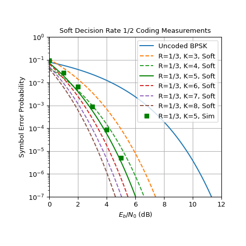
>>> # Compare a collection of simulation results with soft decision
>>> # bounds
>>> SNRdB = np.arange(0,12,.1)
>>> Pb_uc = fec.conv_Pb_bound(1/3,7,[4, 12, 20, 72, 225],SNRdB,2)
>>> Pb_s_third_3 = fec.conv_Pb_bound(1/3,8,[3, 0, 15],SNRdB,1)
>>> Pb_s_third_4 = fec.conv_Pb_bound(1/3,10,[6, 0, 6, 0],SNRdB,1)
>>> Pb_s_third_5 = fec.conv_Pb_bound(1/3,12,[12, 0, 12, 0, 56],SNRdB,1)
>>> Pb_s_third_6 = fec.conv_Pb_bound(1/3,13,[1, 8, 26, 20, 19, 62],SNRdB,1)
>>> Pb_s_third_7 = fec.conv_Pb_bound(1/3,14,[1, 0, 20, 0, 53, 0, 184],SNRdB,1)
>>> Pb_s_third_8 = fec.conv_Pb_bound(1/3,16,[1, 0, 24, 0, 113, 0, 287, 0],SNRdB,1)
>>> Pb_s_half = fec.conv_Pb_bound(1/2,7,[4, 12, 20, 72, 225],SNRdB,1)
>>> plt.figure(figsize=(5,5))
>>> plt.semilogy(SNRdB,Pb_uc)
>>> plt.semilogy(SNRdB,Pb_s_third_3,'--')
>>> plt.semilogy(SNRdB,Pb_s_third_4,'--')
>>> plt.semilogy(SNRdB,Pb_s_third_5,'g')
>>> plt.semilogy(SNRdB,Pb_s_third_6,'--')
>>> plt.semilogy(SNRdB,Pb_s_third_7,'--')
>>> plt.semilogy(SNRdB,Pb_s_third_8,'--')
>>> plt.semilogy([0,1,2,3,4,5],[9.08e-02,2.73e-02,6.52e-03,                                8.94e-04,8.54e-05,5e-6],'gs')
>>> plt.axis([0,12,1e-7,1e0])
>>> plt.title(r'Soft Decision Rate 1/2 Coding Measurements')
>>> plt.xlabel(r'$E_b/N_0$ (dB)')
>>> plt.ylabel(r'Symbol Error Probability')
>>> plt.legend(('Uncoded BPSK','R=1/3, K=3, Soft',                    'R=1/3, K=4, Soft','R=1/3, K=5, Soft',                    'R=1/3, K=6, Soft','R=1/3, K=7, Soft',                    'R=1/3, K=8, Soft','R=1/3, K=5, Sim',                     'Simulation'),loc='upper right')
>>> plt.grid();
>>> plt.show()
>>> # Hard decision rate 1/3 simulation
>>> N_bits_per_frame = 10000
>>> EbN0 = 3
>>> total_bit_errors = 0
>>> total_bit_count = 0
>>> cc2 = fec.FECConv(('11111','11011','10101'),25)
>>> # Encode with shift register starting state of '0000'
>>> state = '0000'
>>> while total_bit_errors < 100:
>>>     # Create 100000 random 0/1 bits
>>>     x = randint(0,2,N_bits_per_frame)
>>>     y,state = cc2.conv_encoder(x,state)
>>>     # Add channel noise to bits, include antipodal level shift to [-1,1]
>>>     yn_soft = dc.cpx_awgn(2*y-1,EbN0-10*np.log10(3),1) # Channel SNR is 10*log10(3) dB less
>>>     yn_hard = ((np.sign(yn_soft.real)+1)/2).astype(int)
>>>     z = cc2.viterbi_decoder(yn_hard.real,'hard')
>>>     # Count bit errors
>>>     bit_count, bit_errors = dc.bit_errors(x,z)
>>>     total_bit_errors += bit_errors
>>>     total_bit_count += bit_count
>>>     print('Bits Received = %d, Bit errors = %d, BEP = %1.2e' %                    (total_bit_count, total_bit_errors,                    total_bit_errors/total_bit_count))
>>> print('*****************************************************')
>>> print('Bits Received = %d, Bit errors = %d, BEP = %1.2e' %                (total_bit_count, total_bit_errors,                total_bit_errors/total_bit_count))
Rate 1/3 Object
kmax =  0, taumax = 0
Bits Received = 9976, Bit errors = 251, BEP = 2.52e-02
*****************************************************
Bits Received = 9976, Bit errors = 251, BEP = 2.52e-02
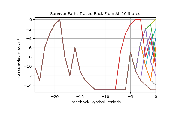
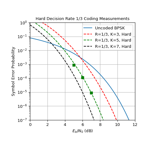
>>> # Compare a collection of simulation results with hard decision
>>> # bounds
>>> SNRdB = np.arange(0,12,.1)
>>> Pb_uc = fec.conv_Pb_bound(1/3,7,[4, 12, 20, 72, 225],SNRdB,2)
>>> Pb_s_third_3_hard = fec.conv_Pb_bound(1/3,8,[3, 0, 15, 0, 58, 0, 201, 0],SNRdB,0)
>>> Pb_s_third_5_hard = fec.conv_Pb_bound(1/3,12,[12, 0, 12, 0, 56, 0, 320, 0],SNRdB,0)
>>> Pb_s_third_7_hard = fec.conv_Pb_bound(1/3,14,[1, 0, 20, 0, 53, 0, 184],SNRdB,0)
>>> Pb_s_third_5_hard_sim = np.array([8.94e-04,1.11e-04,8.73e-06])
>>> plt.figure(figsize=(5,5))
>>> plt.semilogy(SNRdB,Pb_uc)
>>> plt.semilogy(SNRdB,Pb_s_third_3_hard,'r--')
>>> plt.semilogy(SNRdB,Pb_s_third_5_hard,'g--')
>>> plt.semilogy(SNRdB,Pb_s_third_7_hard,'k--')
>>> plt.semilogy(np.array([5,6,7]),Pb_s_third_5_hard_sim,'sg')
>>> plt.axis([0,12,1e-7,1e0])
>>> plt.title(r'Hard Decision Rate 1/3 Coding Measurements')
>>> plt.xlabel(r'$E_b/N_0$ (dB)')
>>> plt.ylabel(r'Symbol Error Probability')
>>> plt.legend(('Uncoded BPSK','R=1/3, K=3, Hard',                    'R=1/3, K=5, Hard', 'R=1/3, K=7, Hard',                    ),loc='upper right')
>>> plt.grid();
>>> plt.show()
>>> # Show the traceback for the rate 1/3 hard decision case
>>> cc2.traceback_plot()
- class sk_dsp_comm.fec_conv.TrellisBranches(Ns)[source]
A structure to hold the trellis states, bits, and input values for both ‘1’ and ‘0’ transitions. Ns is the number of states = \(2^{(K-1)}\).
- class sk_dsp_comm.fec_conv.TrellisNodes(Ns)[source]
A structure to hold the trellis from nodes and to nodes. Ns is the number of states = \(2^{(K-1)}\).
- class sk_dsp_comm.fec_conv.TrellisPaths(Ns, D)[source]
A structure to hold the trellis paths in terms of traceback_states, cumulative_metrics, and traceback_bits. A full decision depth history of all this infomation is not essential, but does allow the graphical depiction created by the method traceback_plot(). Ns is the number of states = \(2^{(K-1)}\) and D is the decision depth. As a rule, D should be about 5 times K.
- sk_dsp_comm.fec_conv.binary(num, length=8)[source]
Format an integer to binary without the leading ‘0b’
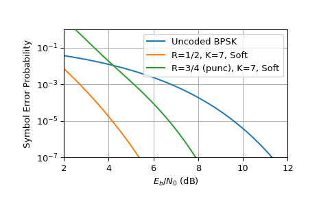
- sk_dsp_comm.fec_conv.conv_Pb_bound(R, dfree, Ck, SNRdB, hard_soft, M=2)[source]
Coded bit error probabilty
Convolution coding bit error probability upper bound according to Ziemer & Peterson 7-16, p. 507
Mark Wickert November 2014
- Parameters
- R: Code rate
- dfree: Free distance of the code
- Ck: Weight coefficient
- SNRdB: Signal to noise ratio in dB
- hard_soft: 0 hard, 1 soft, 2 uncoded
- M: M-ary
Notes
The code rate R is given by \(R_{s} = \frac{k}{n}\). Mark Wickert and Andrew Smit 2018
Examples
>>> import numpy as np
>>> from sk_dsp_comm import fec_conv as fec
>>> import matplotlib.pyplot as plt
>>> SNRdB = np.arange(2,12,.1)
>>> Pb = fec.conv_Pb_bound(1./2,10,[36, 0, 211, 0, 1404, 0, 11633],SNRdB,2)
>>> Pb_1_2 = fec.conv_Pb_bound(1./2,10,[36, 0, 211, 0, 1404, 0, 11633],SNRdB,1)
>>> Pb_3_4 = fec.conv_Pb_bound(3./4,4,[164, 0, 5200, 0, 151211, 0, 3988108],SNRdB,1)
>>> plt.semilogy(SNRdB,Pb)
>>> plt.semilogy(SNRdB,Pb_1_2)
>>> plt.semilogy(SNRdB,Pb_3_4)
>>> plt.axis([2,12,1e-7,1e0])
>>> plt.xlabel(r'$E_b/N_0$ (dB)')
>>> plt.ylabel(r'Symbol Error Probability')
>>> plt.legend(('Uncoded BPSK','R=1/2, K=7, Soft','R=3/4 (punc), K=7, Soft'),loc='best')
>>> plt.grid();
>>> plt.show()