[1]:
import numpy as np
from sk_dsp_comm import sigsys as ss
from sk_dsp_comm import synchronization as sync
from matplotlib import pyplot as plt
Automatic Frequency Control
The module synchronization.py has component classes for implementing AFC. The following example shows how to implement the AFC a quadricorrelator/frequency discriminator class for sample-by-sample processing, as is needed for tracking loop simulation/implementation.
AFC Tracking Loop
[2]:
# Define input signal for AFC
f_clk_afc = 100e3
n = np.arange(100000)
fc = 1000
fm = 100
# Test with amplitude modulation
x_in = (1 + 0.8*np.cos(2*np.pi*fm/f_clk_afc*n))*np.exp(1j*2*np.pi*fc/f_clk_afc*n)
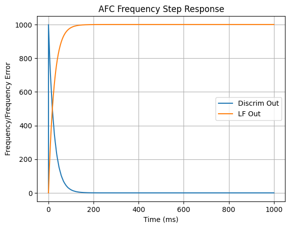
[3]:
Bn_afc = 10
y_d_afc, y_lf_afc, x_out_afc = sync.cbb_afc(x_in, Bn_afc, 1.0, fc_afc=0.0, f_clk_afc=f_clk_afc, afc_open=False)
plt.plot(n/f_clk_afc*1e3,y_d_afc,label='Discrim Out')
plt.plot(n/f_clk_afc*1e3,y_lf_afc,label='LF Out')
# Plot RC lowpass step response theory
# Analog
plt.title(r'AFC Frequency Step Response')
plt.ylabel(r'Frequency/Frequency Error')
plt.xlabel(r'Time (ms)')
plt.legend()
plt.grid();
AFC: ki = 3.999e-04
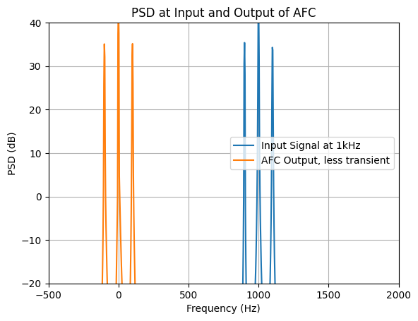
[4]:
Px_in, fx_in = ss.psd(x_in,2**15,f_clk_afc)
plt.plot(fx_in,10*np.log10(Px_in),label='Input Signal at 1kHz')
Px_out, fx_out = ss.psd(x_out_afc[10000:],2**15,f_clk_afc)
plt.plot(fx_out,10*np.log10(Px_out),label='AFC Output, less transient')
plt.title(r'PSD at Input and Output of AFC')
plt.xlabel(r'Frequency (Hz)')
plt.ylabel(r'PSD (dB)')
plt.ylim(-20,40)
plt.xlim(-500,2000)
plt.legend()
plt.grid();