\tableofcontents % These TeX commands run at the start to remove section numbering \renewcommand{\thesection}{\hspace*{-1.0em}} \renewcommand{\thesubsection}{\hspace*{-1.0em}} \renewcommand{\thesubsubsection}{\hspace*{-1.0em}}

%pylab inline
#%matplotlib qt
import sk_dsp_comm.sigsys as ss
import scipy.signal as signal
from IPython.display import Audio, display
from IPython.display import Image, SVG

%pylab is deprecated, use %matplotlib inline and import the required libraries.
Populating the interactive namespace from numpy and matplotlib

pylab.rcParams['savefig.dpi'] = 100 # default 72
#pylab.rcParams['figure.figsize'] = (6.0, 4.0) # default (6,4)
#%config InlineBackend.figure_formats=['png'] # default for inline viewing
%config InlineBackend.figure_formats=['svg'] # SVG inline viewing
#%config InlineBackend.figure_formats=['pdf'] # render pdf figs for LaTeX

import scipy.special as special
import sk_dsp_comm.digitalcom as dc
import sk_dsp_comm.fec_block as block

Block Codes

Block codes take serial source symbols and group them into k-symbol blocks. They then take n-k check symbols to make code words of length n > k. The code is denoted (n,k). The following shows a general block diagram of block encoder.

The block encoder takes k source bits and encodes it into a length n codeword. A block decoder then works in reverse. The length n channel symbol codewords are decoded into the original length k source bits.

Single Error Correction Block Codes

Several block codes are able to correct only one error per block. Two common single error correction codes are cyclic codes and hamming codes. In scikit-dsp-comm there is a module called fec_block.py. This module contains two classes so far: fec_cyclic for cyclic codes and fec_hamming for hamming codes. Each class has methods for encoding, decoding, and plotting theoretical bit error probability bounds.

Cyclic Codes

A (n,k) cyclic code can easily be generated with an n-k stage shift register with appropriate feedback according to Ziemer and Tranter pgs 646 and 647. The following shows a block diagram for a cyclic encoder.

This block diagram can be expanded to larger codes as well. A generator polynomial can be used to determine the position of the binary adders. The previous example uses a generator polynomial of ‘1011’. This means that there is a binary adder after the input, after second shift register, and after the third shift register.

The source symbol length and the channel symbol length can be determined from the number of shift registers \(j\). The length of the generator polynomial is always \(1+j\). In this case we have 3 shift registers, so \(j=3\). We have \(k=4\) source bits and \(n=7\) channel bits. For other shift register lengths, we can use the following equations. \(n=j^2-1\) and \(k = n-j\). The following table (from Ziemer and Peterson pg 429) shows the source symbol length, channel symbol length, and the code rate for various shift register lengths for single error correction codes.

j	k	n	R=k/n
3	4	7	0.57
4	11	15	0.73
5	26	31	0.84
6	57	63	0.90
7	120	127	0.94
8	247	255	0.97
9	502	511	0.98
10	1013	1023	0.99

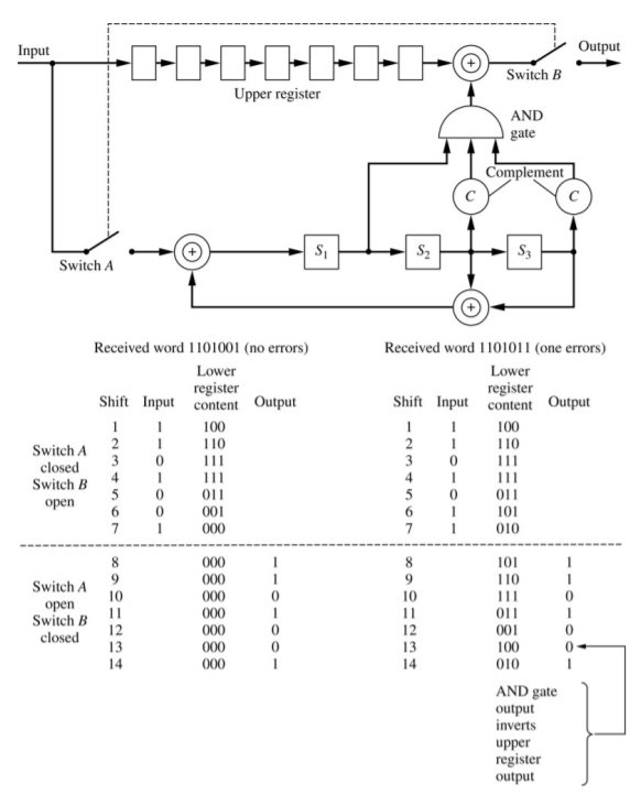
The following block diagram shows a block decoder (from Ziemer and Tranter page 647). The block decoder takes in a codeword of channel symbol length n and decodes it to the original source bits of length k.

The fec_cyclic class can be used to generate a cyclic code object. The cyclic code object can be initialized by a generator polynomial. The length of the generator determines the source symbol length, the channel symbol length, and the rate. The following shows the generator polynomial ‘1011’ considered in the two example block diagrams.

cc1 = block.FECCyclic('1011')

After the cyclic code object cc1 is created, the cc1.cyclic_encoder method can be used to encode source data bits. In the following example, we generate 16 distinct source symbols to get 16 distinct channel symbol codewords using the cyclic_encoder method. The cyclic_encoder method takes an array of source bits as a paramter. The array of source bits must be a length of a multiple of \(k\). Otherwise, the method will throw an error.

# Generate 16 distinct codewords
codewords = zeros((16,7),dtype=int)
x = zeros((16,4))
for i in range(0,16):
    xbin = block.binary(i,4)
    xbin = array(list(xbin)).astype(int)
    x[i,:] = xbin
x = reshape(x,size(x)).astype(int)
codewords = cc1.cyclic_encoder(x)
print(reshape(codewords,(16,7)))

[[0 0 0 0 0 0 0]
 [0 0 0 1 0 1 1]
 [0 0 1 0 1 1 0]
 [0 0 1 1 1 0 1]
 [0 1 0 0 1 1 1]
 [0 1 0 1 1 0 0]
 [0 1 1 0 0 0 1]
 [0 1 1 1 0 1 0]
 [1 0 0 0 1 0 1]
 [1 0 0 1 1 1 0]
 [1 0 1 0 0 1 1]
 [1 0 1 1 0 0 0]
 [1 1 0 0 0 1 0]
 [1 1 0 1 0 0 1]
 [1 1 1 0 1 0 0]
 [1 1 1 1 1 1 1]]

Now, a bit error is introduced into each of the codewords. Then, the codwords with the error are decoded using the cyclic_decoder method. The cyclic_decoder method takes an array of codewords of length \(n\) as a parameter and returns an array of source bits. Even with 1 error introduced into each codeword, All of the original source bits are still decoded properly.

# introduce 1 bit error into each code word and decode
codewords = reshape(codewords,(16,7))
for i in range(16):
    error_pos = i % 6
    codewords[i,error_pos] = (codewords[i,error_pos] +1) % 2
codewords = reshape(codewords,size(codewords))
decoded_blocks = cc1.cyclic_decoder(codewords)
print(reshape(decoded_blocks,(16,4)))

[[0 0 0 0]
 [0 0 0 1]
 [0 0 1 0]
 [0 0 1 1]
 [0 1 0 0]
 [0 1 0 1]
 [0 1 1 0]
 [0 1 1 1]
 [1 0 0 0]
 [1 0 0 1]
 [1 0 1 0]
 [1 0 1 1]
 [1 1 0 0]
 [1 1 0 1]
 [1 1 1 0]
 [1 1 1 1]]

The following example generates many random source symbols. It then encodes the symbols using the cyclic encoder. It then simulates a channel by adding noise. It then implements hard decisions on each of the incoming bits and puts the received noisy bits into the cyclic decoder. Source bits are then returned and errors are counted until 100 bit errors are received. Once 100 bit errors are received, the bit error probability is calculated. This code can be run at a variety of SNRs and with various code rates.

cc1 = block.FECCyclic('101001')
N_blocks_per_frame = 2000
N_bits_per_frame = N_blocks_per_frame*cc1.k
EbN0 = 6
total_bit_errors = 0
total_bit_count = 0

while total_bit_errors < 100:
    # Create random 0/1 bits
    x = randint(0,2,N_bits_per_frame)
    y = cc1.cyclic_encoder(x)
    # Add channel noise to bits and scale to +/- 1
    yn = dc.cpx_awgn(2*y-1,EbN0-10*log10(cc1.n/cc1.k),1) # Channel SNR is dB less
    # Scale back to 0 and 1
    yn = ((sign(yn.real)+1)/2).astype(int)
    z = cc1.cyclic_decoder(yn)
    # Count bit errors
    bit_count, bit_errors = dc.bit_errors(x,z)
    total_bit_errors += bit_errors
    total_bit_count += bit_count
    print('Bits Received = %d, Bit errors = %d, BEP = %1.2e' %\
          (total_bit_count, total_bit_errors,\
           total_bit_errors/total_bit_count))
print('*****************************************************')
print('Bits Received = %d, Bit errors = %d, BEP = %1.2e' %\
      (total_bit_count, total_bit_errors,\
       total_bit_errors/total_bit_count))

Bits Received = 52000, Bit errors = 44, BEP = 8.46e-04

Bits Received = 104000, Bit errors = 100, BEP = 9.62e-04
*****************************************************
Bits Received = 104000, Bit errors = 100, BEP = 9.62e-04

There is a function in the fec_block module called block_single_error_Pb_bound that can be used to generate the theoretical bit error probability bounds for single error correction block codes. Measured bit error probabilities from the previous example were recorded to compare to the bounds.

SNRdB = arange(0,12,.1)
#SNRdB = arange(9.4,9.6,0.1)
Pb_uc = block.block_single_error_Pb_bound(3,SNRdB,False)
Pb_c_3 = block.block_single_error_Pb_bound(3,SNRdB)
Pb_c_4 = block.block_single_error_Pb_bound(4,SNRdB)
Pb_c_5 = block.block_single_error_Pb_bound(5,SNRdB)
figure(figsize=(5,5))
semilogy(SNRdB,Pb_uc,'k-')
semilogy(SNRdB,Pb_c_3,'c--')
semilogy(SNRdB,Pb_c_4,'m--')
semilogy(SNRdB,Pb_c_5,'g--')
semilogy([4,5,6,7,8,9],[1.44e-2,5.45e-3,2.37e-3,6.63e-4,1.33e-4,1.31e-5],'cs')
semilogy([5,6,7,8],[4.86e-3,1.16e-3,2.32e-4,2.73e-5],'ms')
semilogy([5,6,7,8],[4.31e-3,9.42e-4,1.38e-4,1.15e-5],'gs')
axis([0,12,1e-10,1e0])
title('Cyclic code BEP')
xlabel(r'$E_b/N_0$ (dB)')
ylabel(r'Bit Error Probability')
legend(('Uncoded BPSK','(7,4), hard',\
        '(15,11), hard', '(31,26), hard',\
        '(7,4) sim', '(15,11) sim', \
        '(31,26) sim'),loc='lower left')
grid();

These plots show that the simulated bit error probability is very close to the theoretical bit error probabilites.

Hamming Code

Hamming codes are another form of single error correction block codes. Hamming codes use parity-checks in order to generate and decode block codes. The code rates of Hamming codes are generated the same way as cyclic codes. In this case a parity-check length of length \(j\) is chosen, and n and k are calculated by \(n=2^j-1\) and \(k=n-j\). Hamming codes are generated first by defining a parity-check matrix \(H\). The parity-check matrix is a j x n matrix containing binary numbers from 1 to n as the columns. For a \(j=3\) (\(k=4\), \(n=7\)) Hamming code. The parity-check matrix starts out as the following:

\begin{equation} \mathbf{H} = \left[\begin{array} {rrr} 0 & 0 & 0 & 1 & 1 & 1 & 1\\ 0 & 1 & 1 & 0 & 0 & 1 & 1\\ 1 & 0 & 1 & 0 & 1 & 0 & 1 \end{array}\right] \end{equation}

The parity-chekc matrix can be reordered to provice a systematic code by interchanging the columns to create an identity matrix on the right side of the matrix. In this case, this is done by interchangeing columsn 1 and 7, columns 2 and 6, and columsn 4 and 5. The resulting parity-check matrix is the following.

\begin{equation} \mathbf{H} = \left[\begin{array} {rrr} 1 & 1 & 0 & 1 & 1 & 0 & 0\\ 1 & 1 & 1 & 0 & 0 & 1 & 0\\ 1 & 0 & 1 & 1 & 0 & 0 & 1 \end{array}\right] \end{equation}

Next, a generator matrix \(G\) is created by restructuring the parity-check matrix. The \(G\) matrix is gathered from the \(H\) matrix through the following relationship.

\begin{equation} \mathbf{G} = \left[\begin{array} {rrr} I_k & ... & H_p \end{array}\right] \end{equation}

where \(H_p\) is defined as the transpose of the first k columns of H. For this example we arrive at the following \(G\) matrix. G always ends up being a k x n matrix.

\begin{equation} \mathbf{G} = \left[\begin{array} {rrr} 1 & 0 & 0 & 0 & 1 & 1 & 1\\ 0 & 1 & 0 & 0 & 1 & 1 & 0\\ 0 & 0 & 1 & 0 & 0 & 1 & 1\\ 0 & 0 & 0 & 1 & 1 & 0 & 1 \end{array}\right] \end{equation}

Codewords can be generated by multiplying a source symbol matrix by the generator matrix.

\begin{equation} codeword = xG \end{equation}

Where the codeword is a column vector of length \(n\) and x is a row vector of length \(n\). This is the basic operation of the encoder. The decoder is slightly more complicated. The decoder starts by taking the parity-check matrix \(H\) and multiplying it by the codeword column vector. This gives the “syndrome” of the block. The syndrome tells us whether or not there is an error in the codeword. If no errors are present, the syndrome will be 0. If there is an error in the codeword, the syndrome will tell us which bit has the error.

\begin{equation} S = H \cdot codeword \end{equation}

If the syndrome is nonzero, then it can be used to correct the error bit in the codeword. After that, the original source blocks can be decoded from the codewords by the following equation.

\begin{equation} source = R\cdot codeword \end{equation}

Where \(R\) is a k x n matrix where R is made up of a k x k identity matrix and a k x n-k matrix of zeros. Again, the Hamming code is only capable of correcting one error per block, so if more than one error is present in the block, then the syndrome cannot be used to correct the error.

The hamming code class can be found in the fec_block module as fec_hamming. Hamming codes are sometimes generated using generator polynomials just like with cyclic codes. This is not completely necessary, however, if the previously described process is used. This process simply relies on choosing a number of parity bits and then systematic single-error correction hamming codes are automatically generated. The following will go through an example of a \(j=3\) (\(k=4\), \(n=7\)) hamming code.

Hamming Block Code Class Definition:

hh1 = block.FECHamming(3)

\(k\) and \(n\) are calculated form the number of parity checks \(j\) and can be accessed by hh1.k and hh1.n. The \(j\) x \(n\) parity-check matrix \(H\) and the \(k\) x \(n\) generator matrix \(G\) can be accessed by hh1.H and hh1.G. These are exactly as described previously.

print('k = ' + str(hh1.k))
print('n = ' + str(hh1.n))
print('H = \n' + str(hh1.H))
print('G = \n' + str(hh1.G))

k = 4
n = 7
H =
[[1 1 0 1 1 0 0]
 [1 1 1 0 0 1 0]
 [1 0 1 1 0 0 1]]
G =
[[1 0 0 0 1 1 1]
 [0 1 0 0 1 1 0]
 [0 0 1 0 0 1 1]
 [0 0 0 1 1 0 1]]

The fec_hamming class has an encoder method called hamm_encoder. This method works the same way as the cyclic encoder. It takes an array of source bits with a length that is a multiple of \(k\) and returns an array of codewords. This class has another method called hamm_decoder which can decode an array of codewords. The array of codewords must have a length that is a multiple of \(n\). The following example generates random source bits, encodes them using a hamming encoder, simulates transmitting them over a channel, uses hard decisions after the receiver to get a received array of codewords, and decodes the codewords using the hamming decoder. It runs until it counds 100 bit errors and then calculates the bit error probability. This can be used to simulate hamming codes with different rates (different numbers of parity checks) at different SNRs.

hh1 = block.FECHamming(5)
N_blocks_per_frame = 20000
N_bits_per_frame = N_blocks_per_frame*hh1.k
EbN0 = 8
total_bit_errors = 0
total_bit_count = 0


while total_bit_errors < 100:
    # Create random 0/1 bits
    x = randint(0,2,N_bits_per_frame)
    y = hh1.hamm_encoder(x)
    # Add channel noise to bits and scale to +/- 1
    yn = dc.cpx_awgn(2*y-1,EbN0-10*log10(hh1.n/hh1.k),1) # Channel SNR is dB less
    # Scale back to 0 and 1
    yn = ((sign(yn.real)+1)/2).astype(int)
    z = hh1.hamm_decoder(yn)
    # Count bit errors
    bit_count, bit_errors = dc.bit_errors(x,z)
    total_bit_errors += bit_errors
    total_bit_count += bit_count
    print('Bits Received = %d, Bit errors = %d, BEP = %1.2e' %\
          (total_bit_count, total_bit_errors,\
           total_bit_errors/total_bit_count))
print('*****************************************************')
print('Bits Received = %d, Bit errors = %d, BEP = %1.2e' %\
      (total_bit_count, total_bit_errors,\
       total_bit_errors/total_bit_count))

Bits Received = 520000, Bit errors = 4, BEP = 7.69e-06

Bits Received = 1040000, Bit errors = 16, BEP = 1.54e-05

Bits Received = 1560000, Bit errors = 29, BEP = 1.86e-05

Bits Received = 2080000, Bit errors = 34, BEP = 1.63e-05

Bits Received = 2600000, Bit errors = 46, BEP = 1.77e-05

Bits Received = 3120000, Bit errors = 69, BEP = 2.21e-05

Bits Received = 3640000, Bit errors = 72, BEP = 1.98e-05

Bits Received = 4160000, Bit errors = 84, BEP = 2.02e-05

Bits Received = 4680000, Bit errors = 86, BEP = 1.84e-05

Bits Received = 5200000, Bit errors = 102, BEP = 1.96e-05
*****************************************************
Bits Received = 5200000, Bit errors = 102, BEP = 1.96e-05

The fec_block.block_single_error_Pb_bound function can also be used to generate the bit error probability bounds for hamming codes. The following example generates theoretical bit error probability bounds for hamming codes and compares it with simulated bit error probabilities from the previous examples.

SNRdB = arange(0,12,.1)
Pb_uc = block.block_single_error_Pb_bound(3,SNRdB,False)
Pb_c_3 = block.block_single_error_Pb_bound(3,SNRdB)
Pb_c_4 = block.block_single_error_Pb_bound(4,SNRdB)
Pb_c_5 = block.block_single_error_Pb_bound(5,SNRdB)
figure(figsize=(5,5))
semilogy(SNRdB,Pb_uc,'k-')
semilogy(SNRdB,Pb_c_3,'c--')
semilogy(SNRdB,Pb_c_4,'m--')
semilogy(SNRdB,Pb_c_5,'g--')
semilogy([5,6,7,8,9,10],[6.64e-3,2.32e-3,5.25e-4,1.16e-4,1.46e-5,1.19e-6],'cs')
semilogy([5,6,7,8,9],[4.68e-3,1.19e-3,2.48e-4,3.6e-5,1.76e-6],'ms')
semilogy([5,6,7,8,9],[4.42e-3,1.11e-3,1.41e-4,1.43e-5,6.73e-7],'gs')
axis([0,12,1e-10,1e0])
title('Hamming code BEP')
xlabel(r'$E_b/N_0$ (dB)')
ylabel(r'Bit Error Probability')
legend(('Uncoded BPSK','(7,4), hard',\
        '(15,11), hard', '(31,26), hard',\
        '(7,4) sim', '(15,11) sim', \
        '(31,26) sim'),loc='lower left')
grid();

Multiple Error Correction Block Codes

Other block codes are capable of correcting multiple errors in blocks. Golay Codes, Bose_Chaudhuri-Hocquenghem (BCH) Codes, and Reed-Solomon Codes are all capable of correcting multiple errors. These codes have not been developed yet, but they will be the next codes to be added to the fec_block module.

Golay Code

Golay codes are capable of correcting three errors in a block of 23 symbols. Golay codes are one of the few known “perfect” codes where all error patterns with hamming weight \(t\) or less and no error patters with weight greater than \(t\) are correctable using a minimum-distance maximum-likelihood decoder. Golay codes are discussed in detail in Ziemer and Peterson pgs 448-450.

Bose-Chaudhuri-Hocquenghem (BCH) Codes

BCH codes are very important because they exist for a wide range of rates, can achieve significant coding gain, and decoders can be implemented even at high speeds. BCH codes are described in detail in Ziemer and Peterson pgs 436-444.

Reed-Solomon Codes

RS codes are nonbinary BCH codes that use input and output alphabets having \(2^m\) symbols, {\(0,1,2,...,2^m-1\)}. Block length is \(n=2^m-1\) and can be extended to \(n=2^m\) or \(n=2^m+1\). Reed-Solomon codes are useful in burst communications Reed-Solomon Codes are discussed in detail in Ziemer and Peterson pgs 444-447.