%pylab inline
import sk_dsp_comm.sigsys as ss
import sk_dsp_comm.fir_design_helper as fir_d
import sk_dsp_comm.iir_design_helper as iir_d
import sk_dsp_comm.multirate_helper as mrh
import scipy.signal as signal
from IPython.display import Audio, display
from IPython.display import Image, SVG

%pylab is deprecated, use %matplotlib inline and import the required libraries.
Populating the interactive namespace from numpy and matplotlib

%config InlineBackend.figure_formats=['svg'] # SVG inline viewing

Multirate Signal Processing Using multirate_helper

In this section the classes multirate_FIR and multirate_IIR, found in the module sk_dsp_comm.multirate_helper, are discussed with the aim of seeing how they can be used to filter, interpolate (upsample and filter), and decimate (filter and downsample) discrete time signals. Fundamentally the processing consists of two elements: (1) and upsampler or downsampler and (2) a lowpass filter.

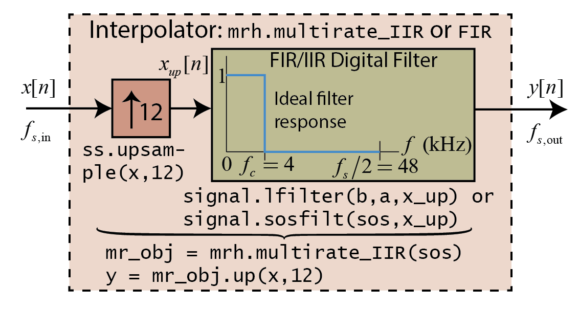
Fundamentally this modules provides classes to change the sampling rate by an integer factor, either up, interpolation or down, decimation, with integrated filtering to supress spectral images or aliases, respectively. The top level block diagram of the interpolator and decimator are given in the following two figures. The frequencies given in the figures assume that the interpolator is rate chainging from 8 ksps to 96 ksps (\(L=12\)) and the decimator is rate changing from 96 ksps to 8 ksps (\(M=12\)). This is for example purposes only. The FIR/IIR filter cutoff frequency will in general be \(f_c = f_\text{s,out}/(2L)\) for the decimator and \(f_c = f_\text{s,in}/(2M)\). The primitives to implement the classes are available in sk_dsp_comm.sigsys and scipy.signal.

Image('300ppi/Interpolator_Top_Level@300ppi.png',width='60%')

Image('300ppi/Decimator_Top_Level@300ppi.png',width='60%')

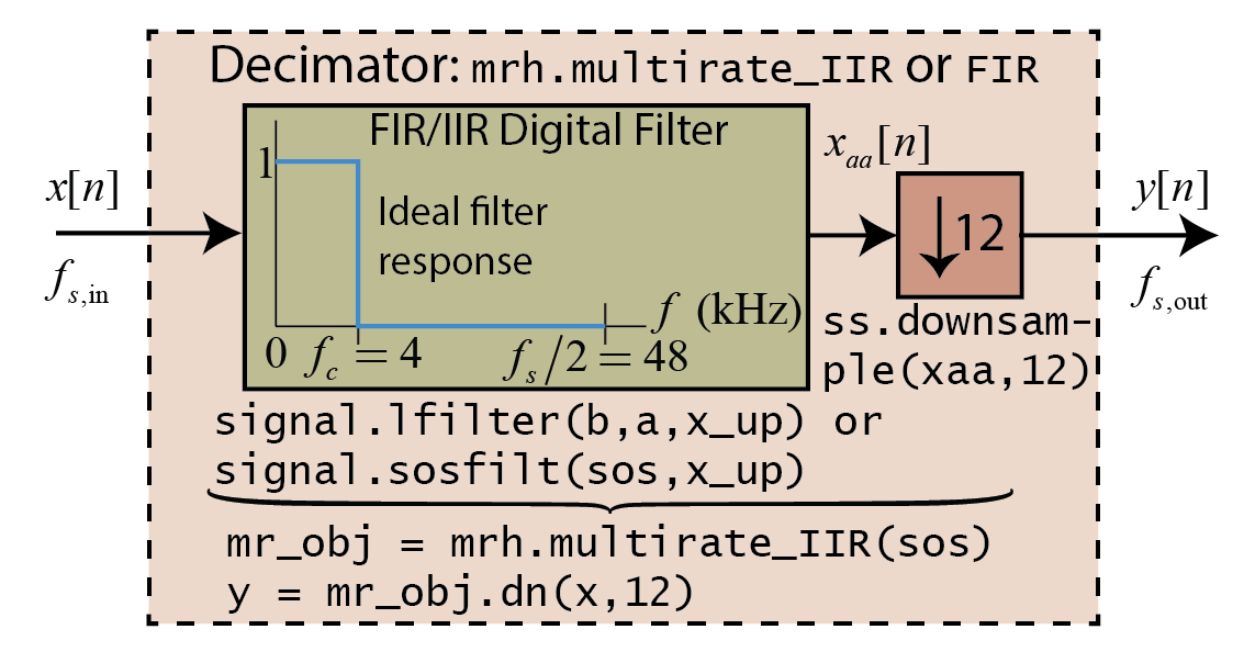
The upsample block, shown above with arrow pointing up and integer \(L=12\) next to the arrow, takes the input sequence and produces the output sequence by inserting \(L-1\) (as shown here 11) zero samples between each input sample. The downsample block, shown above with arrow pointing down and integer \(M=12\) next to the arrow, takes the input sequence and retains at the output sequence every \(M\)th (as shown here 12th) sample.

The impact of these blocks in the frequency domain is a little harder to explain. In words, the spectrum at the output of the upsampler is compressed by the factor \(L\), such that it will contain \(L\) spectral images, including the fundamental image centered at \(f = 0\), evenly spaced up to the sampling \(f_s\). Overall the spectrum of \(x_\text{up}[n]\) is of course periodic with respect to the sampling rate. The lowpass filter interpolates signal sample values from the non-zero samples where the zero samples reside. It is this interpolation that effectively removed or suppresses the spectral images outside the interval \(|f| > f_s/(2L)\).

For the downsampler the input spectrum is stretched along the frequency axis by the factor \(M\), with aliasing from frequency bands outside \(|f| < f_s/(2M)\). To avoid aliasing the lowpass filter blocks input signals for \(f > f_s/(2M)\).

To get started using the module you will need an import similar to:

import sk_dsp_comm.multirate_helper as mrh

The rate_change Class

We start with the description of a third class, mrh.rate_change, which is simplistic, offering little user interaction, but automatically designs the required lowpass filter you see in the above block diagrams. Below is a table which describes this class:

Image('300ppi/Multirate_Table1@300ppi.png',width='85%')

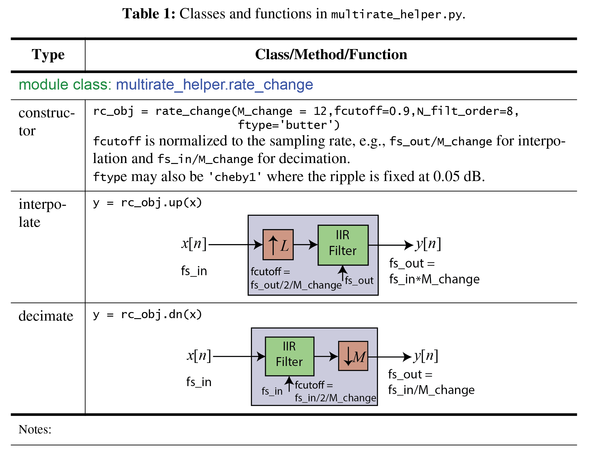
This class is used in the analog modulation demos for the ECE 4625/5625 Chapter 3 Jupyter notebook. Using this class you can quickly create a interpolation or decimation block with the necessary lowpass filter automatically designed and implemented. Fine tuning of the filter is limited to choosing the filter order and the cutoff frequency as a fraction of the signal bandwidth given the rate change integer, \(L\) or \(M\). The filter type is also limited to Butterworth or Chebyshev type 1 having passband ripple of 0.05 dB.

A Simple Example

Pass a sinusoidal signal through an \(L=4\) interpolator. Verify that spectral images occur with the use of the interpolation lowpass filter.

fs_in = 8000
M = 4
fs_out = M*fs_in
rc1 = mrh.rate_change(M) # Rate change by 4
n = arange(0,1000)
x = cos(2*pi*1000/fs_in*n)
x_up = ss.upsample(x,4)
y = rc1.up(x)

Time Domain

subplot(211)
stem(n[500:550],x_up[500:550]);
ylabel(r'$x_{up}[n]$')
title(r'Upsample by $L=4$ Output')
#ylim(-100,-10)
subplot(212)
stem(n[500:550],y[500:550]);
ylabel(r'$y[n]$')
xlabel(r'')
title(r'Interpolate by $L=4$ Output')
#ylim(-100,-10)
tight_layout()

• Clearly the lowpass interpolation filter has done a good job of filling in values for the zero samples

Frequency Domain

subplot(211)
psd(x_up,2**10,fs_out);
ylabel(r'PSD (dB)')
title(r'Upsample by $L=4$ Output')
ylim(-100,-10)
subplot(212)
psd(y,2**10,fs_out);
ylabel(r'PSD (dB)')
title(r'Interpolate by $L=4$ Output')
ylim(-100,-10)
tight_layout()

• The filtering action of the LPF does its best to suppress the images at 7000, 9000, and 15000 Hz.

The multirate_FIR Class

With this class you implement an object that can filter, interpolate, or decimate a signal. Additionally support methods drill into the characteristics of the lowpass filter at the heart of the processing block. To use this class the user must supply FIR filter coefficients that implement a lowpass filter with cutoff frequency appropriate for the desired interpolation of decimation factor. The module sk_dsp_com.FIR_design_helper is capable of delivering the need filter coefficients array. See FIR design helper notes for multirate filter design examples.

With FIR coefficients in hand it is an easy matter to create an multirate FIR object capable of filtering, interpolation, or decimation. The details of the class interface are given in Table 2 below.

Image('300ppi/Multirate_Table2@300ppi.png',width='85%')

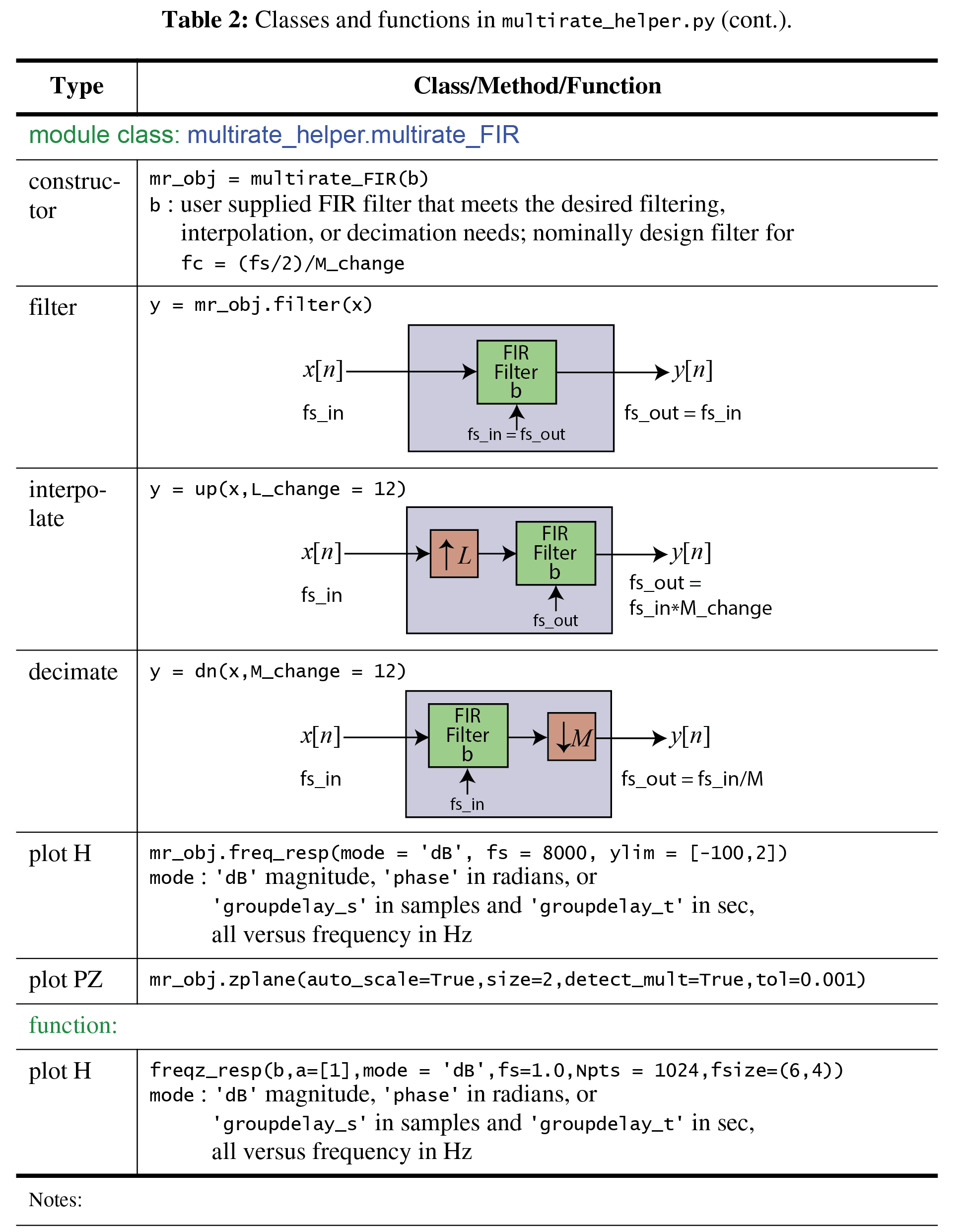
Notice that the class also provides a means to obtain frequency response plots and pole-zero plots directly from the instantiated multirate objects.

FIR Interpolator Design Example

Here we take the earlier lowpass filter designed to interpolate a signal being upsampled from \(f_{s1} = 8000\) kHz to \(f_{s2} = 96\) kHz. The upsampling factor is \(L = f_{s2}/f_{s1} = 12\). The ideal interpolation filter should cutoff at \(f_{s1}/2 = f_{s2}/(2\cdot 12) = 8000/2 = 4000\) Hz.

Recall the upsampler (y = ss.upsampler(x, L)) inserts \(L-1\) samples between each input sample. In the frequency domain the zero insertion replicates the input spectrum on \([0,f_{s1}/2]\) \(L\) times over the interval \([0,f_{s2}]\) (equivalently \(L/2\) times on the inteval \([0f_{s2}/2]\). The lowpass interpolation filter serves to removes the images above \(f_{s2}/(2L)\) in the frequency domain and in so doing filling in the zeros samples with waveform interpolants in the time domain.

# Design the filter core for an interpolator used in changing the sampling rate from 8000 Hz
# to 96000 Hz
b_up = fir_d.fir_remez_lpf(3300,4300,0.5,60,96000)
# Create the multirate object
mrh_up = mrh.multirate_FIR(b_up)

As an input consider a sinusoid at 1 kHz and observe the interpolator output spectrum compared with the input spectrum.

# Sinusoidal test signal
n = arange(10000)
x = cos(2*pi*1000/8000*n)
# Interpolate by 12 (upsample by 12 followed by lowpass filter)
y = mrh_up.up(x,12)

# Plot the results
subplot(211)
psd(x,2**12,8000);
title(r'1 KHz Sinusoid Input to $L=12$ Interpolator')
ylabel(r'PSD (dB)')
ylim([-100,0])
subplot(212)
psd(y,2**12,12*8000)
title(r'1 KHz Sinusoid Output from $L=12$ Interpolator')
ylabel(r'PSD (dB)')
ylim([-100,0])
tight_layout()

In the above spectrum plots notice that images of the input 1 kHz sinusoid are down \(\simeq 60\) dB, which is precisely the stop band attenuation provided by the interpolation filter. The variation is due to the stopband ripple.

The multirate_IIR Class

With this class, as with multirate_FIR you implement an object that can filter, interpolate, or decimate a signal. The filter in this case is a user supplied IIR filter in second-order sections (sos) form. Additionally support methods drill into the characteristics of the lowpass filter at the heart of the procssing block. The module sk_dsp_com.IIR_design_helper is capable of delivering the need filter coefficients array. See IIR design helper notes for multirate filter design examples.

With IIR coefficients in hand it is an easy matter to create an multirate IIR object capable of filtering, interpolation, or decimation. The details of the class interface are given in Table 3 below.

Image('300ppi/Multirate_Table3@300ppi.png',width='85%')

IIR Decimator Design Example

Whan a signal is decimated the signal is first lowpass filtered then downsampled. The lowpass filter serves to prevent aliasing as the sampling rate is reduced. Downsampling by \(M\) (y = ss.downsample(x, M)) removes \(M-1\) sampling for every \(M\) sampling input or equivalently retains one sample out of \(M\). The lowpass prefilter has cutoff frequency equal to the folding frequency of the output sampling rate, i.e., \(f_c = f_{s2}/2\). Note avoid confusion with the project requirements, where the decimator is needed to take a rate \(f_{s2}\) signal back to \(f_{s1}\), let the input sampling rate be \(f_{s2} = 96000\) HZ and the output sampling rate be \(f_{s1} = 8000\) Hz. The input sampling rate is \(M\) times the output rate, i.e., \(f_{s2} = Mf_{s1}\), so you design the lowpass filter to have cutoff \(f_c = f_{s2}/(2\cdot L)\).

ECE 5625 Important Observation: In the coherent SSB demodulator of Project 1, the decimator can be conveniently integrated with the lowpass filter that serves to remove the double frequency term.

In the example that follows a Chebyshev type 1 lowpass filter is designed to have cutoff around 4000 Hz. A sinusoid is used as a test input signal at sampling rate 96000 Hz.

# Design the filter core for a decimator used in changing the
# sampling rate from 96000 Hz to 8000 Hz
b_dn, a_dn, sos_dn = iir_d.IIR_lpf(3300,4300,0.5,60,96000,'cheby1')
# Create the multirate object
mrh_dn = mrh.multirate_IIR(sos_dn)
mrh_dn.freq_resp('dB',96000)
title(r'Decimation Filter Frequency Response - Magnitude');

• Note the Chebyshev lowpass filter design above is very efficient compared with the 196-tap FIR lowpass designed for use in the interpolator. It is perhaps a better overall choice. The FIR has linear phase and the IIR filter does not, but for the project this is not really an issue.

As an input consider a sinusoid at 1 kHz and observe the interpolator output spectrum compared with the input spectrum.

# Sinusoidal test signal
n = arange(100000)
x = cos(2*pi*1000/96000*n)
# Decimate by 12 (lowpass filter followed by downsample by 12)
y = mrh_dn.dn(x,12)

# Plot the results
subplot(211)
psd(x,2**12,96000);
title(r'1 KHz Sinusoid Input to $M=12$ Decimator')
ylabel(r'PSD (dB)')
ylim([-100,0])
subplot(212)
psd(y,2**12,8000)
title(r'1 KHz Sinusoid Output from $M=12$ Decimator')
ylabel(r'PSD (dB)')
ylim([-100,0])
tight_layout()